Build complex primitive cells

In this tutorial, we demonstrate how to construct complex primitive cells using the python-based modeling tools. The scripts are located at examples/prim_cell/model/graphene_rect.py and examples/prim_cell/model/graphene_nr.py. TBPLaS offers two sets of modeling tools: Python-based and Cython-based. Python-based tools are designed for models of moderate size, and all work at the primitive cell level. Here are the summary of the Python-based tools:

• reshape_prim_cell

• extend_prim_cell

• apply_pbc

• remove_orbitals

• remove_hopping

• trim

• spiral_prim_cell

• make_hetero_layer

• merge_prim_cell

reshape_prim_cell() reshapes the primitive cell to new lattice vectors. extend_prim_cell() replicates the primitive cell along \(a\), \(b\), and \(c`\) directions. apply_pbc() is a method of the PrimitiveCell class, and makes a periodic primitive cell non-periodic by removing hopping terms to neighbouring cells along given directions. We will show the usage of these functions by constructing graphene nano-ribbon with armchair and zigzag edges from the primitive cell.

remove_orbitals() and remove_hopping() are also methods of the PrimitiveCell class, and remove an orbital or hopping term from the primitive cell, respectively. Dangling orbitals and hopping terms may remain in the cell after the removal, and can be trimmed with the trim() method. We will show the usage of these functions by constructing a large graphene cell with vacancies.

spiral_prim_cell(), make_hetero_layer() and merge_prim_cell() are functions specially designed for building hetero-structures. Their usage will be discussed in Build hetero-structure.

Construct graphene nano-ribbon

Make rectangular cell

To make graphene nano-ribbons we need the rectangular primitive cell. We can built it from scratch as:

import math
import tbplas as tb

# Generate lattice vectors
sqrt3 = math.sqrt(3)
a = 2.46
cc_bond = sqrt3 / 3 * a
vectors = tb.gen_lattice_vectors(sqrt3 * cc_bond, 3 * cc_bond)

# Create cell and add orbitals
rect_cell = tb.PrimitiveCell(vectors)
rect_cell.add_orbital((0, 0))
rect_cell.add_orbital((0, 2 / 3.))
rect_cell.add_orbital((1 / 2., 1 / 6.))
rect_cell.add_orbital((1 / 2., 1 / 2.))

# Add hopping terms
rect_cell.add_hopping([0, 0], 0, 2, -2.7)
rect_cell.add_hopping([0, 0], 2, 3, -2.7)
rect_cell.add_hopping([0, 0], 3, 1, -2.7)
rect_cell.add_hopping([0, 1], 1, 0, -2.7)
rect_cell.add_hopping([1, 0], 3, 1, -2.7)
rect_cell.add_hopping([1, 0], 2, 0, -2.7)

# Plot the cell
rect_cell.plot()

But the function reshape_prim_cell() offers a more convenient approach. In the figure we show the relation of the lattices of rectangular cell to diamond-shaped cell:

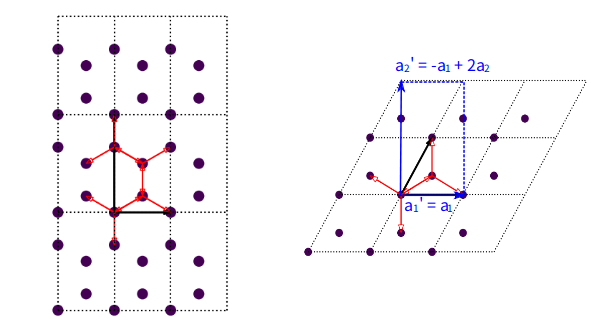
Rectangular and diamond-shaped primitive cells of monolayer graphene. The rectangular cell is indicated with blue rectangle, with lattice vectors (\(a_1\prime\) and \(a_2\prime\)) shown as solid arrows.

It is clear that:

• \(a_1\prime = a_1\)

• \(a_2\prime = -a_1 + 2a_2\)

• \(a_3\prime = a_3\)

The last relation is not explicitly shown in the figure, but required by TBPLaS since all primitive cells are implemented as three-dimensional internally. From the relation we can construct the rectangular cell as:

import numpy as np
import tbplas as tb

# Import diamond-shaped primitive cell from materials repository
cell = tb.make_graphene_diamond()

# Define conversion matrix of lattice vectors
lat_sc = np.array([[1, 0, 0], [-1, 2, 0], [0, 0, 1]])

# Reshape the primitive cell
rect_cell = tb.reshape_prim_cell(cell, lat_sc)

# Plot the cell
rect_cell.plot()

Here cell is the diamond-shaped primitive cell. lat_sc is the conversion matrix of lattice vectors. By changing the conversion matrix we can reshape the primitive cell to different shapes, which is particular useful for constructing hetero-structures. We will show it in Build hetero-structure.

Extend rectangular cell

To produce a graphene nano-ribbon with desired width we need to extend the rectangular cell. We do this by calling the extend_prim_cell() function:

gnr = tb.extend_prim_cell(rect_cell, dim=(3, 3, 1))
gnr.plot()

Here we extend the rectangular cell along \(a\) and \(b\) directions by 3 times through the dim parameter. The output is shown as below:

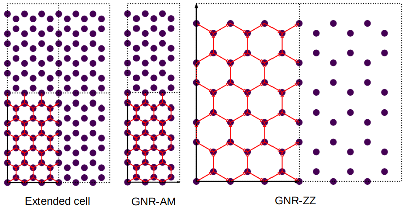
Extend rectangular primitive cell and graphene nano-ribbon with armchair edges (GNR-AM) or zigag edges (GNR-ZZ).

Impose non-periodic boundary condition

The extend rectangular cell is periodic along \(a\) and \(b\) directions, i.e., it is two-dimensional. But graphene nano-ribbons are one-dimensional. We can impose non-periodic boundary conditions along specific direction by calling the apply_pbc() method:

gnr.apply_pbc(pbc=(False, True, False))
gnr.plot(with_conj=False)

Here we enforce the cell to be periodic only along \(b\) direction, yielding a nano-ribbon with armchair edges, as shown in the middle panel of the figure shown above. We can also enforce the cell to be periodic along \(a\) direction to make a nano-ribbon with zigzag edges:

gnr = tb.extend_prim_cell(rect_cell, dim=(3, 3, 1))
gnr.apply_pbc(pbc=(True, False, False))
gnr.plot(with_conj=False)

Note that apply_pbc() does not return a new primitive cell as other functions. Instead, the original primitive cell is modified. So we need to extend the rectangular cell again before calling apply_pbc().

Finally we can evaluate the band structure of armchair-edged nano-ribbon with:

k_points = np.array([
    [0.0, -0.5, 0.0],
    [0.0, 0.0, 0.0],
    [0.0, 0.5, 0.0],
])
k_label = ["X", "G", "X"]
k_path, k_idx = tb.gen_kpath(k_points, [40, 40])
k_len, bands = gnr.calc_bands(k_path)
vis = tb.Visualizer()
vis.plot_bands(k_len, bands, k_idx, k_label)

For zigzag-edged nano-ribbon, replace k_points with:

k_points = np.array([
    [-0.5, 0.0, 0.0],
    [0.0, 0.0, 0.0],
    [0.5, 0.0, 0.0],
])

The band structures should look like:

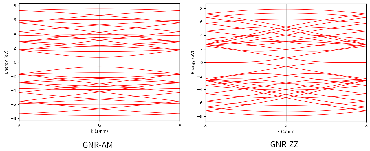
Band structures of armchair and zigag-edged graphene nano-ribbons.

It is consistent with the literature: zigzag-edged graphene nano-ribbons are always metallic, while armchair-edged graphene nano-ribbons can be either metallic or semi-conducting.

Remove orbitals and hopping terms

Remove orbitals

To demonstrate the usage of remove_orbitals() and remove_hopping() we need to import the diamond-shaped primitive cell of graphene and extend it by 3 times along \(a\) and \(b\) directions:

import tbplas as tb

cell = tb.make_graphene_diamond()
cell = tb.extend_prim_cell(cell, dim=(3, 3, 1))
cell.plot(with_conj=False)

The output is shown in the right panel of the figure:

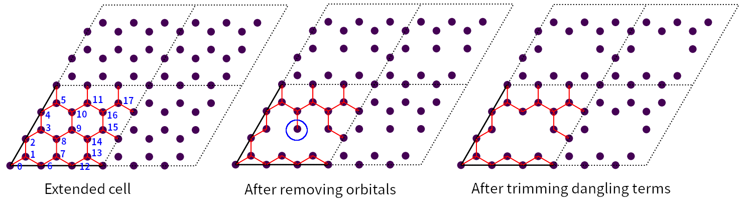
Structure of extended graphene primitive cell before and after removing orbitals and after trimming dangling terms. Blue circle indicates the dangling orbital.

We remove orbital #8 and #14 with the following commands:

cell.remove_orbitals([8, 14])
orb_to_remove = [8, 14]
for i, orb in enumerate(sorted(orb_to_remove)):
    cell.remove_orbital(orb - i)
cell.plot(with_conj=False)

The output is shown in the middle panel. Obviously, orbital #8 and #14 have been removed. However, orbital #9 becomes dangling, since there is only one hopping term associated with it. We can remove the orbital and associated hopping terms with the trim() method:

cell.trim()
cell.plot(with_conj=False)

Note that trim() does not return a new primitive cell, but modifies the original cell in-place. The output is shown in the right panel. The dangling orbital and hopping term are removed after calling the function.

Remove hopping terms

From the extended cell we can also remove hopping terms, e.g. \((0, 0) \rightarrow (0, 0), i=3, j=8\) and \((0, 0) \rightarrow (0, 0), i=8, j=9\) with the following commands:

cell = tb.make_graphene_diamond()
cell = tb.extend_prim_cell(cell, dim=(3, 3, 1))
cell.remove_hopping(rn=(0, 0), orb_i=3, orb_j=8)
cell.remove_hopping(rn=(0, 0), orb_i=8, orb_j=9)
cell.plot(with_conj=False)

The output is shown in the left panel of the figure:

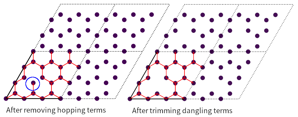
Structure of extended graphene primitive cell after removing hopping and after trimming dangling terms. Blue circle indicates the dangling orbital.

Similarly, we can remove dangling terms in the same way:

cell.trim()
cell.plot(with_conj=False)

The output is shown in the right panel.