Spin-orbital coupling
In this tutorial, we show how to introduce spin-orbital coupling (SOC) into the primitive cell
taking \(\mathrm{MoS_2}\) as the example. We will consider the intra-atom SOC in the form of
\(H^{soc} = \lambda \mathbf{L}\cdot\mathbf{S}\). For this type of SOC, TBPLaS offers the
SOC class for evaluating the matrix elements of \(\mathbf{L}\cdot\mathbf{S}\) in the
direct product basis \(|l\rangle\otimes|s\rangle\). We prefer this basis set because it does
not involve the evaluation of Clebsch-Gordan coefficients. There is also a SOCTable class
which contains the pre-calculated matrix elements ans can be utilized in the same approach as
SOC. The corresponding script can be found at examples/prim_cell/soc_ls.py. Other types
of SOC, e.g., Kane-Mele inter-atom SOC or Rashba SOC, can be found in the tbplas.materials.graphene
module. In principle, all types of SOC can be implemented with doubling the orbitals and add hopping
terms between the spin-polarized orbitals. We begin with importing the necessary packages:
import numpy as np

import tbplas as tb
Create cell without SOC
Similar to the case of Slater-Koster formulation, we build the primitive cell without SOC as
 1# Lattice vectors from ref. 3
 2vectors = np.array([
 3    [3.1600000, 0.000000000, 0.000000000],
 4    [-1.579999, 2.736640276, 0.000000000],
 5    [0.000000000, 0.000000000, 3.1720000000],
 6])
 7
 8# Orbital coordinates
 9coord_mo = [0.666670000, 0.333330000, 0.5]
10coord_s1 = [0.000000000, -0.000000000, 0.0]
11coord_s2 = [0.000000000, -0.000000000, 1]
12orbital_coord = [coord_mo for _ in range(5)]
13orbital_coord.extend([coord_s1 for _ in range(3)])
14orbital_coord.extend([coord_s2 for _ in range(3)])
15orbital_coord = np.array(orbital_coord)
16
17# Orbital labels
18mo_orbitals = ("Mo:dz2", "Mo:dzx", "Mo:dyz", "Mo:dx2-y2", "Mo:dxy")
19s1_orbitals = ("S1:px", "S1:py", "S1:pz")
20s2_orbitals = ("S2:px", "S2:py", "S2:pz")
21orbital_label = mo_orbitals + s1_orbitals + s2_orbitals
22
23# Orbital energies
24# Parameters from ref. 3
25orbital_energy = {"dz2": -1.512, "dzx": 0.419, "dyz": 0.419,
26                  "dx2-y2": -3.025, "dxy": -3.025,
27                  "px": -1.276, "py": -1.276, "pz": -8.236}
28
29# Create the primitive cell and add orbitals
30cell = tb.PrimitiveCell(lat_vec=vectors, unit=tb.ANG)
31for i, label in enumerate(orbital_label):
32    coord = orbital_coord[i]
33    energy = orbital_energy[label.split(":")[1]]
34    cell.add_orbital(coord, energy=energy, label=label)
35
36# Get hopping terms in the nearest approximation
37neighbors = tb.find_neighbors(cell, a_max=2, b_max=2, max_distance=0.32)
38
39# Add hopping terms
40sk = tb.SK()
41for term in neighbors:
42    i, j = term.pair
43    label_i = cell.get_orbital(i).label
44    label_j = cell.get_orbital(j).label
45    hop = calc_hop(sk, term.rij, label_i, label_j)
46    cell.add_hopping(term.rn, i, j, hop)
where we also need to define the lattice vectors, orbital positions, labels and energies. The
on-site energies are taken from the
reference. It should
be noted that we must add the atom label to the orbital label in line 18-20, in order to distinguish
the orbitals located on the same atom when adding SOC. Then we create the cell, add orbitals and
hopping terms in line 29-46. The calc_hop function is defined as:
 1def calc_hop(sk: tb.SK, rij: np.ndarray, label_i: str, label_j: str) -> complex:
 2    """
 3    Evaluate the hopping integral <i,0|H|j,r> for single layer MoS2.
 4
 5    Reference:
 6    [1] https://www.mdpi.com/2076-3417/6/10/284
 7    [2] https://journals.aps.org/prb/abstract/10.1103/PhysRevB.88.075409
 8    [3] https://iopscience.iop.org/article/10.1088/2053-1583/1/3/034003/meta
 9    Note ref. 2 and ref. 3 share the same set of parameters.
10
11    :param sk: SK instance
12    :param rij: displacement vector from orbital i to j in nm
13    :param label_i: label of orbital i
14    :param label_j: label of orbital j
15    :return: hopping integral in eV
16    """
17    # Parameters from ref. 3
18    v_pps, v_ppp = 0.696, 0.278
19    v_pds, v_pdp = -2.619, -1.396
20    v_dds, v_ddp, v_ddd = -0.933, -0.478, -0.442
21
22    lm_i = label_i.split(":")[1]
23    lm_j = label_j.split(":")[1]
24
25    return sk.eval(r=rij, label_i=lm_i, label_j=lm_j,
26                   v_pps=v_pps, v_ppp=v_ppp,
27                   v_pds=v_pds, v_pdp=v_pdp,
28                   v_dds=v_dds, v_ddp=v_ddp, v_ddd=v_ddd)
which shares much in common with the calc_hop function in Slater-Koster formulation.
Add SOC
We fine the following function for adding SOC:
 1def add_soc(cell: tb.PrimitiveCell) -> tb.PrimitiveCell:
 2    """
 3    Add spin-orbital coupling to the primitive cell.
 4
 5    :param cell: primitive cell to modify
 6    :return: primitive cell with soc
 7    """
 8    # Double the orbitals and hopping terms
 9    cell = tb.merge_prim_cell(cell, cell)
10
11    # Add spin notations to the orbitals
12    num_orb_half = cell.num_orb // 2
13    num_orb_total = cell.num_orb
14    for i in range(num_orb_half):
15        label = cell.get_orbital(i).label
16        cell.set_orbital(i, label=f"{label}:up")
17    for i in range(num_orb_half, num_orb_total):
18        label = cell.get_orbital(i).label
19        cell.set_orbital(i, label=f"{label}:down")
20
21    # Add SOC terms
22    # Parameters from ref. 3
23    soc_lambda = {"Mo": 0.075, "S1": 0.052, "S2": 0.052}
24    soc = tb.SOC()
25    for i in range(num_orb_total):
26        label_i = cell.get_orbital(i).label.split(":")
27        atom_i, lm_i, spin_i = label_i
28
29        # Since the diagonal terms of l_dot_s is exactly zero in the basis of
30        # real atomic orbitals (s, px, py, pz, ...), and the conjugate terms
31        # are handled automatically in PrimitiveCell class, we need to consider
32        # the upper triangular terms only.
33        for j in range(i+1, num_orb_total):
34            label_j = cell.get_orbital(j).label.split(":")
35            atom_j, lm_j, spin_j = label_j
36
37            if atom_j == atom_i:
38                soc_intensity = soc.eval(label_i=lm_i, spin_i=spin_i,
39                                         label_j=lm_j, spin_j=spin_j)
40                soc_intensity *= soc_lambda[atom_j]
41                if abs(soc_intensity) >= 1.0e-15:
42                    # CAUTION: if the lower triangular terms are also included
43                    # in the loop, SOC coupling terms will be double counted
44                    # and the results will be wrong!
45                    try:
46                        energy = cell.get_hopping((0, 0, 0), i, j)
47                    except tb.PCHopNotFoundError:
48                        energy = 0.0
49                    energy += soc_intensity
50                    cell.add_hopping((0, 0, 0), i, j, energy)
51    return cell
In this function, we firstly double the orbitals and hopping terms in the primitive cell using the
merge_prim_cell() function in line 9, in order to yield the direct product basis
\(|l\rangle\otimes|s\rangle\). Then we add spin notations, namely up and down, to the
orbital labels in line 12-19. After that, we define the SOC intensity \(\lambda\) for Mo and S,
taking data from the reference.
Then we create an instance from the SOC class, and loop over the upper-triangular orbital
paris to add SOC. Note that the SOC terms are added for orbital pairs located on the same atom by
checking their atom labels in line 37. The matrix element of \(\mathbf{L}\cdot\mathbf{S}\) in
the direct product basis \(|l\rangle\otimes|s\rangle\) is evaluated with the eval function
of SOC class in line 38-39, taking the orbital and spin notations as input. If the
corresponding hopping term already exists, then SOC will be added to it. Otherwise, a new hopping
term will be created, as shown in line 45-50. Finally, the new cell with SOC is returned.
Check the results
We check the primitive cell we have just created by calculating its band structure:
 1# Add soc
 2cell = add_soc(cell)
 3
 4# Plot band structure to compare with Fig 5 in Ref 2.(without SOC) and Ref 3.(within SOC)
 5k_points = np.array([
 6    [0.0, 0.0, 0.0],
 7    [1. / 2, 0.0, 0.0],
 8    [1. / 3, 1. / 3, 0.0],
 9    [0.0, 0.0, 0.0],
10])
11k_label = ["G", "M", "K", "G"]
12k_path, k_idx = tb.gen_kpath(k_points, [40, 40, 40])
13prefix = "mos2_soc" if with_soc else "mos2"
14k_len, bands = tb.calc_bands(cell, k_path, prefix=prefix)
15tb.Visualizer().plot_bands(k_len, bands, k_idx, k_label))
The results are shown in the left panel, consistent with the band structure in the right panel taken from the reference, where the splitting of VBM at \(\mathbf{K}\)-point is perfectly reproduced.
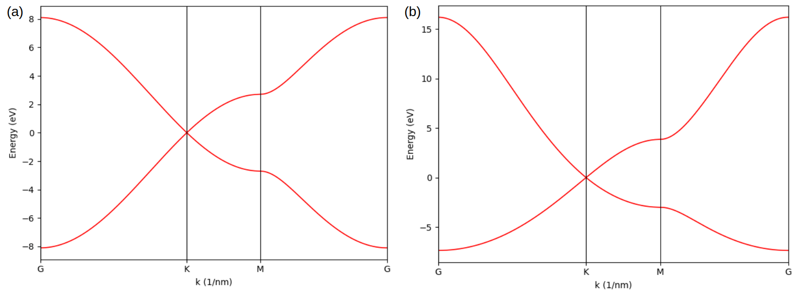
Band structure of MoS2 (a) created in this tutorial and (b) taken from the reference.