Spin texture
In this tutorial, we demonstrate the usage of SpinTexture class by calculating the spin
texture and spin-resolved band structure of graphene with Rashba and Kane-Mele spin-orbital coupling.
The spin texture is defined as the the expectation of Pauli operator \(\sigma_i\), which can be
considered as a function of band index \(n\) and \(\mathbf{k}\)-point
where \(i \in {x, y, z}\) are components of the Pauli operator. The spin texture can be evaluated
for given band index \(n\) or fixed energy. The script is located at examples/prim_cell/spin_texture/spin_texture.py.
As in other tutorials, we begin with importing the tbplas package:
from typing import List

import numpy as np
import matplotlib.pyplot as plt

import tbplas as tb
Spin texture
We define the following function for calculating the spin texture:
 1def calc_spin_texture(cell: tb.PrimitiveCell,
 2                      prefix: str = "kane_mele",
 3                      ib: int = 0,
 4                      spin_major: bool = True) -> None:
 5    # Sigma_z on a fine grid
 6    spin_texture = tb.SpinTexture(cell)
 7    spin_texture.config.prefix = f"{prefix}_sigma_z"
 8    spin_texture.config.k_points = 2 * (tb.gen_kmesh((240, 240, 1)) - 0.5)
 9    spin_texture.config.k_points[:, 2] = 0.0
10    spin_texture.config.spin_major = spin_major
11    spin_data = spin_texture.calc_spin_texture()
12    plot_sigma_z_band(spin_data, ib)
13
14    # Sigma_x and sigma_y on a coarse grid
15    spin_texture.config.prefix = f"{prefix}_sigma_xy"
16    spin_texture.config.k_points = 2 * (tb.gen_kmesh((48, 48, 1)) - 0.5)
17    spin_texture.config.k_points[:, 2] = 0.0
18    spin_data = spin_texture.calc_spin_texture()
19    plot_sigma_xy_band(spin_data, ib)
20    plot_sigma_xy_eng(spin_data)
Firstly, we create a SpinTexture object. Then we define the prefix of data files, the k-points
and the order of spin-polarized orbitals. To plot the expectation of \(\sigma_i\) as function of
\(\mathbf k\)-point, we need to generate a uniform mesh grid in the Brillouin zone. As the
gen_kmesh() function generates k-grid on \([0, 1]\), we need to multiply the result by
a factor of 2, then extract 1 from it such that the k-grid will be on \([-1, 1]\) which is enough to
cover the first Brillouin zone. After that, we call the calc_spin_texture method to calculate the spin
texture. The result is a SpinData object, which contains the Cartesian coordinates of k-points,
the energies and the expectation of \(\sigma_x\), \(\sigma_y\) and \(\sigma_z\).
The expectation of \(\sigma_z\) can be visualized as scalar field. We achieve this by calling the
plot_sigma_z_band function. The result is shown in the left panel of Fig. 1. The expectation of
\(\sigma_x\) and \(\sigma_y\) can be visualized simultaneously as vector field. we call the
plot_sigma_xy_band function to visualize \(\sigma_x\) and \(\sigma_y\) of specific band,
and plot_sigma_xy_eng to visualize that of specific energy range. The result is shown in the middle
and right panels of Fig. 1, where the signature of Rashba spin-orbital coupling is clearly demonstrated.
The functions to visualize the results are defined as:
 1def plot_sigma_z_band(spin_data: tb.SpinData, ib: int = 0) -> None:
 2    """
 3    Plot expectation of sigma_z of specific band as scalar field of kx and ky.
 4    :param spin_data: spin texture produced of SpinTexture calculator
 5    :param ib: band index
 6    :return: None
 7    """
 8    # Data aliases
 9    kpt_cart = spin_data.kpt_cart
10    sigma_z = spin_data.sigma_z[:, ib]
11
12    # Plot expectation of sigma_z.
13    vis = tb.Visualizer()
14    vis.plot_scalar(x=kpt_cart[:, 0], y=kpt_cart[:, 1], z=sigma_z, scatter=True,
15                    num_grid=(480, 480), cmap="jet", with_colorbar=True)
16
17
18def plot_sigma_xy_band(spin_data: tb.SpinData, ib: int = 0) -> None:
19    """
20    Plot expectation of sigma_x and sigma_y of specific band as vector field of
21    kx and ky.
22    :param spin_data: spin texture produced of SpinTexture calculator
23    :param ib: band index
24    :return: None
25    """
26    # Data aliases
27    kpt_cart = spin_data.kpt_cart
28    sigma_x = spin_data.sigma_x[:, ib]
29    sigma_y = spin_data.sigma_y[:, ib]
30
31    # Plot expectation of sigma_z.
32    vis = tb.Visualizer()
33    # Plot expectation of sigma_x and sigma_y.
34    vis.plot_vector(x=kpt_cart[:, 0], y=kpt_cart[:, 1], u=sigma_x, v=sigma_y,
35                    cmap="jet", with_colorbar=True)
36
37
38def plot_sigma_xy_eng(spin_data: tb.SpinData,
39                      e_min: float = -2,
40                      e_max: float = -1.9) -> None:
41    """
42    Plot expectation of sigma_x and sigma_y of specific energy range as vector
43    field of kx and ky.
44    :param spin_data: spin texture produced of SpinTexture calculator
45    :param e_min: lower bound of energy range in eV
46    :param e_max: upper bound of energy range in eV
47    :return: None
48    """
49    # Data aliases
50    bands = spin_data.bands
51    kpt_cart = spin_data.kpt_cart
52    sigma_x = spin_data.sigma_x
53    sigma_y = spin_data.sigma_y
54
55    # Extract spin texture of specific energy range
56    e_min, e_max = -2, -1.9
57    ik_selected, sigma_x_selected, sigma_y_selected = [], [], []
58    for i_k in range(bands.shape[0]):
59        idx = np.where((bands[i_k] >= e_min)&(bands[i_k] <= e_max))[0]
60        ik_selected.extend([i_k for _ in idx])
61        sigma_x_selected.extend(sigma_x[i_k, idx])
62        sigma_y_selected.extend(sigma_y[i_k, idx])
63
64    # Plot expectation of sigma_x and sigma_y.
65    vis = tb.Visualizer()
66    vis.plot_vector(x=kpt_cart[ik_selected, 0], y=kpt_cart[ik_selected, 1],
67                    u=sigma_x_selected, v=sigma_y_selected, cmap="jet",
68                    with_colorbar=True)
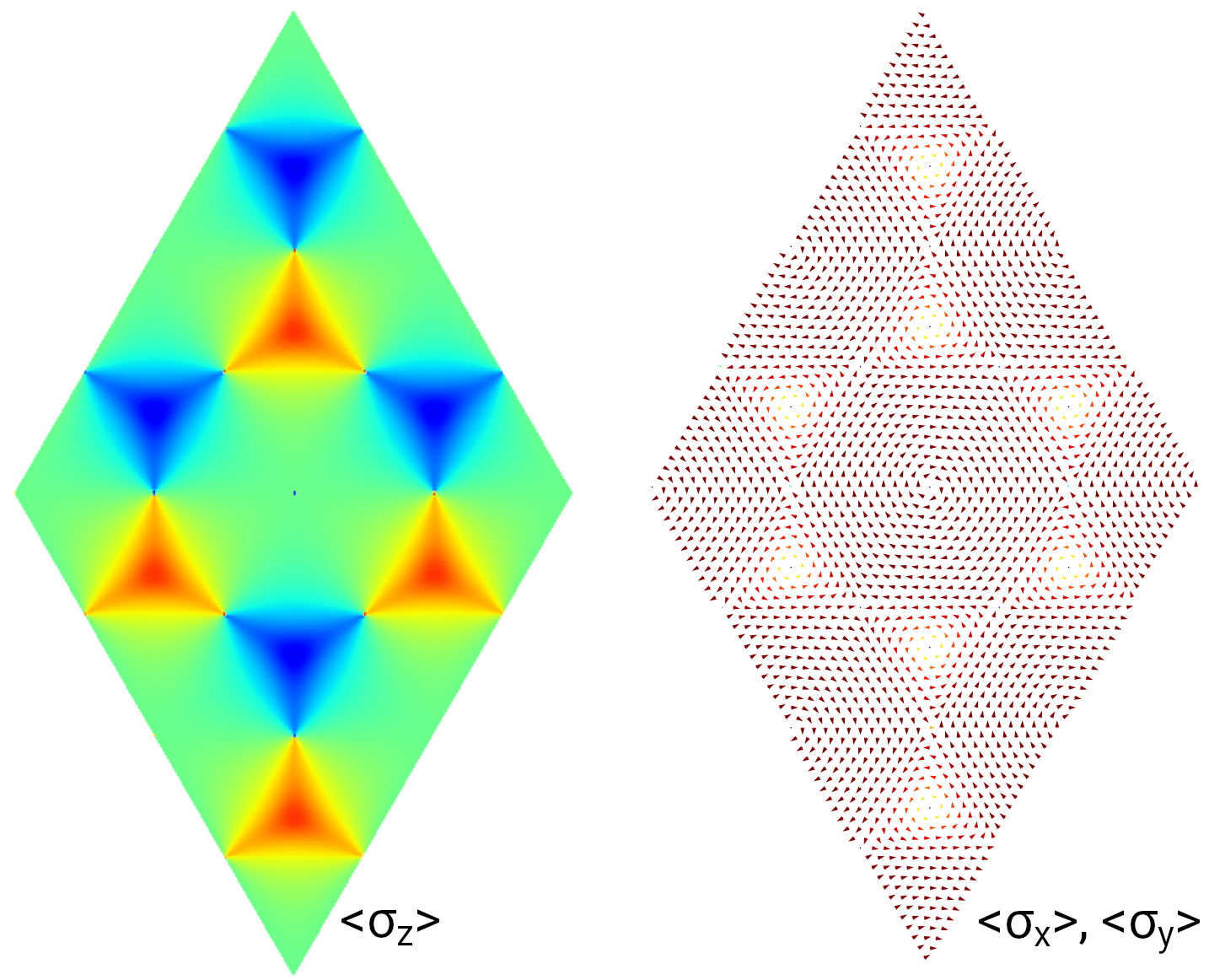
Spin texture of Kane-Mele model. (Left) Expectation of \(\sigma_z\) of 0th band. (Middle) Expectation of \(\sigma_x\) and \(\sigma_y\) of 0th band. (Right) Expectation of \(\sigma_x\) and \(\sigma_y\) of \([-2, -1.9]\) eV.
Spin-resolved band structure
Spin-resolved band structure can be evaluated in the same approach as spin texture. The only difference is that the k-points should be a path connecting high-symmetric k-points in the first Brillouin zone, rather than a regular mesh grid. We define the following function to calculate the spin-resolved band structure:
 1def calc_fat_band(cell: tb.PrimitiveCell,
 2                  prefix: str = "kane_mele",
 3                  spin_major: bool = True) -> None:
 4    # Generate k-path
 5    k_points = np.array([
 6        [0.0, 0.0, 0.0],    # Gamma
 7        [0.5, 0.0, 0.0],    # M
 8        [2./3, 1./3, 0.0],  # K
 9        [0.0, 0.0, 0.0],    # Gamma
10        [1./3, 2./3, 0.0],  # K'
11        [0.5, 0.5, 0.0],    # M'
12        [0.0, 0.0, 0.0],    # Gamma
13    ])
14    k_label = [r"$\Gamma$", "M", "K", r"$\Gamma$",
15               r"$K^{\prime}$", r"$M^{\prime}$", r"$\Gamma$"]
16    k_path, k_idx = tb.gen_kpath(k_points, [40, 40, 40, 40, 40, 40])
17
18    # Evaluate spin texture (including energies)
19    spin_texture = tb.SpinTexture(cell)
20    spin_texture.config.prefix = f"{prefix}_fat_band"
21    spin_texture.config.k_points = k_path
22    spin_texture.config.spin_major = spin_major
23    spin_data = spin_texture.calc_spin_texture()
24
25    # Plot fat band
26    plot_fat_band(spin_data, k_idx, k_label, "z")
The function for visualizing the results is defined as:
 1def plot_fat_band(spin_data: tb.SpinData,
 2                  k_idx: np.ndarray,
 3                  k_label: List[str],
 4                  component: str = "z") -> None:
 5    """
 6    Plot spin-resolved band structure.
 7    :param spin_data: spin texture produced of SpinTexture calculator
 8    :param k_idx: indices of high-symmetric k-points
 9    :param k_label: labels of high-symmetric k-points
10    :param component: component of sigma
11    :return: None
12    """
13    # Data aliases
14    bands = spin_data.bands
15    kpt_cart = spin_data.kpt_cart
16    if component == "x":
17        projection = spin_data.sigma_x
18    elif component == "y":
19        projection = spin_data.sigma_y
20    else:
21        projection = spin_data.sigma_z
22
23    # Evaluate k_len
24    k_len = np.zeros(kpt_cart.shape[0])
25    for i in range(1, kpt_cart.shape[0]):
26        dk = kpt_cart[i] - kpt_cart[i-1]
27        k_len[i] = k_len[i-1] + np.linalg.norm(dk)
28
29    # Plot fat band
30    for ib in range(bands.shape[1]):
31        plt.scatter(k_len, bands[:, ib], c=projection[:, ib], s=5.0, cmap="jet")
32    for x in k_len[k_idx]:
33        plt.axvline(x, color="k", linewidth=0.8, linestyle="-")
34    for y in (-2.0, -1.9):
35        plt.axhline(y, color="k", linewidth=1.0, linestyle=":")
36    plt.xlim(k_len[0], k_len[-1])
37    plt.xticks(k_len[k_idx], k_label)
38    plt.ylabel("Energy (t)")
39    plt.colorbar(label=fr"$\langle\sigma_{component}\rangle$")
40    plt.show()
The spin-resolved band structure for \(\sigma_z\) is shown in Fig. 2, which is consistent with Fig. 1, i.e., zero on \(\Gamma\)-\(M\) and non-zero on \(M\)-\(K\) paths.
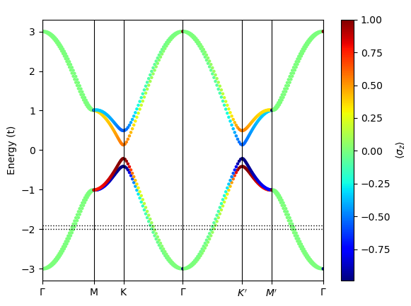
Spin-resolved band structure of Kane-Mele model. Horizontal dashed lines indicate the energy range for plotting spin texture in the right panel of Fig. 1.
Orbital order
The order of spin-polarized orbitals determines how the spin-up and spin-down components are extracted from the
eigenstates. There are two popular orders: spin-major and orbital-major. For example, there are two \(p_z\)
orbitals in the two-band model of monolayer graphene in the spin-unpolarized case, which can be denoted as
\(\{\phi_1, \phi_2\}\). When spin has been taken into consideration, the orbitals become
\(\{\phi_1^{\uparrow}, \phi_2^{\uparrow}, \phi_1^{\downarrow}, \phi_2^{\downarrow}\}\). In spin-major order
they are sorted as \([\phi_1^{\uparrow}, \phi_2^{\uparrow}, \phi_1^{\downarrow}, \phi_2^{\downarrow}]\),
while in orbital-major order they are sorted as
\([\phi_1^{\uparrow}, \phi_1^{\downarrow}, \phi_2^{\uparrow}, \phi_2^{\downarrow}]\). In the C++ backend
of SpinTexture class, the spin-up and spin-down components are extracted as:
 1size_t num_orb_half = num_orbitals / 2;
 2auto seq_up = Eigen::seq(0, num_orb_half - 1, 1);
 3auto seq_down = Eigen::seq(num_orb_half, num_orbitals - 1, 1);
 4if (!spin_major) {
 5    seq_up = Eigen::seq(0, num_orbitals - 2, 2);
 6    seq_down = Eigen::seq(1, num_orbitals - 1, 2);
 7}
 8// ...
 9Eigen::VectorXcd spin_up(num_orb_half); // half size
10Eigen::VectorXcd spin_down(num_orb_half); // half size
11// ...
12spin_up = eigenstates(seq_up, ib);
13spin_down = eigenstates(seq_down, ib);
If the spin-polarized orbitals follow other user-defined orders, the users should modify the
SpinTexture::calc_spin_texture C++ function to correctly extract the spin-up and spin-down
components.