Interfaces

In this tutorial, we shown how to use the interfaces to build the primitive cell from the output of Wannier90 and LAMMPS. The scripts can be found at examples/interface. We begin with importing the necessary packages:

import numpy as np
import matplotlib.pyplot as plt
from ase import io

import tbplas as tb

For LAMMPS, we need the ase library to read in the structure. So it must be installed before starting this tutorial. For Wannier90, no other libraries are required.

Wannier90

The wan2pc() function can read in the output of Wannier90, namely seedname_centres.xyz, seedname_hr.dat, seedname.win and seedname_wsvec.dat, where seedname is the shared prefix of the files, centres.xyz contains the positions of the Wannier functions, hr.dat contains the on-site energies and hopping terms, win is the input file of Wannier90, and wsvec.dat contains information the Wigner-Seitz cell. Only the seedname is required as input. We demonstrate the usage of this function by constructing the 8-orbital primitive cell of graphene and evaluating its band structure:

cell = tb.wan2pc("graphene", hop_eng_cutoff=0.0)
k_points = np.array([
    [0.0, 0.0, 0.0],
    [1./3, 1./3, 0.0],
    [1./2, 0.0, 0.0],
    [0.0, 0.0, 0.0],
])
k_label = ["G", "K", "M", "G"]
k_path, k_idx = tb.gen_kpath(k_points, [40, 40, 40])
k_len, bands = tb.calc_bands(cell, k_path)

num_bands = bands.shape[1]
for i in range(num_bands):
    plt.plot(k_len, bands[:, i], color="r", linewidth=1.0)
for idx in k_idx:
    plt.axvline(k_len[idx], color="k", linewidth=1.0)
plt.xlim((0, np.amax(k_len)))
plt.xticks(k_len[k_idx], k_label)
plt.xlabel("k / (1/nm)")
plt.ylabel("Energy (eV)")
plt.tight_layout()
plt.show()

The output is shown in the left panel, where the Dirac cone at \(\mathbf{K}\)-point is perfectly reproduced.

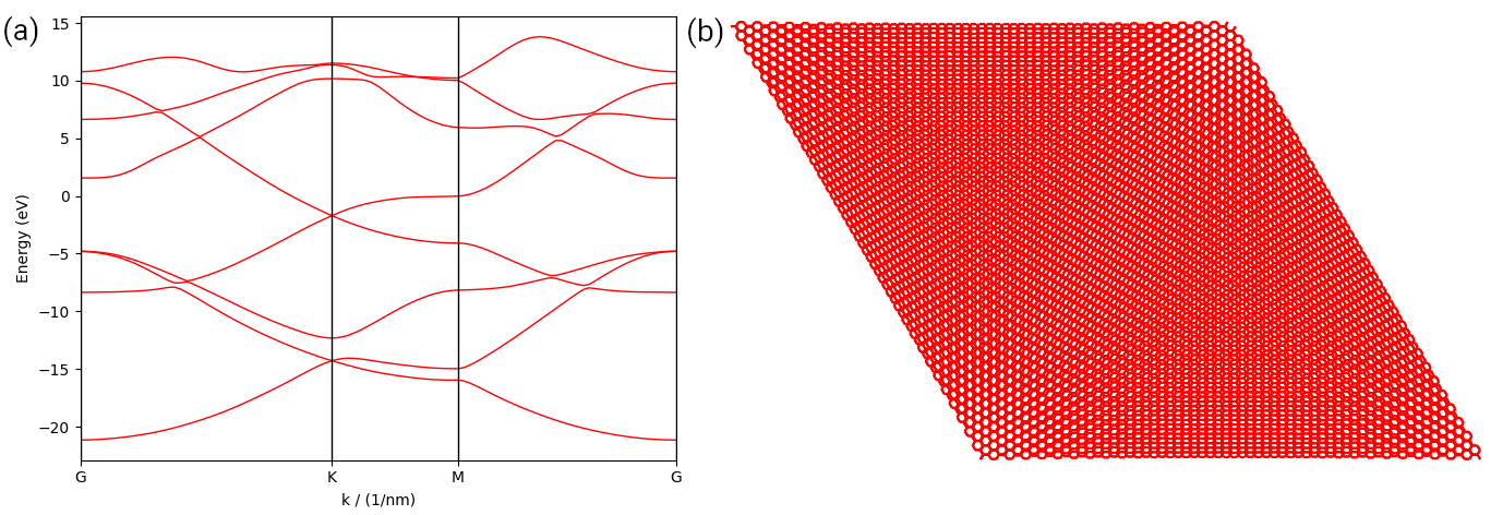
(a) Band structure of monolayer graphene imported from the output of Wannier90. (b) Plot of a large bilayer graphene primitive cell imported from the output of LAMMPS.

LAMMPS

Unlike Wannier90, the output of LAMMPS contains only the atomic positions. So we must add the orbitals and hopping terms manually. We show this by constructing a large bilayer graphene primitive cell:

# Read the last image of lammps dump
atoms = io.read("struct.atom", format="lammps-dump-text", index=-1)

# Get cell lattice vectors in Angstroms
lattice_vectors = atoms.cell

# Create the cell
prim_cell = tb.PrimitiveCell(lat_vec=atoms.cell, unit=tb.ANG)

# Add orbitals
for atom in atoms:
    prim_cell.add_orbital(atom.scaled_position)

# Find hopping neighbors up to 0.145 nm
neighbors = tb.find_neighbors(prim_cell, a_max=1, b_max=1, max_distance=0.145)

# Add hopping terms
for term in neighbors:
    prim_cell.add_hopping(term.rn, term.pair[0], term.pair[1], energy=-2.7)

# Plot the cell
prim_cell.plot(with_cells=False, with_orbitals=False, hop_as_arrows=False)

In line 2 we read in the structure with the read function of ase.io module. Then we extract the lattice vectors from the cell attribute of ase Atoms class and create the primitive cell in line 5-8. After that, we loop over the atoms in the structure and add one \(p_z\) orbital for each atom in line 11-12. The fractional coordinate of the orbital can be extracted from the scaled_position attribute of ase Atom class. Then we call the find_neighbors() function to find the orbital pairs within hopping distance of 0.145 nm (length of C-C bond) in line 15. Finally, we add the hopping terms according to the orbital pairs in line 18-19 and plot the cell in line 22. The output is shown in the right panel of the figure.