Response functions

In this tutorial, we show how to calculate the response functions of primitive cell, namely dynamic polarization, dielectric function and optical (AC) conductivity, using the Lindhard class. The corresponding script is examples/prim_cell/lindhard.py. Lindhard requires the energies and wave functions from exact diagonalization, so its application is limited to primitive cells of small or moderate size. For large models, the tight-binding propagation method (TBPM) is recommended, which will be discussed in Properties from TBPM. Before beginning the tutorial, we import all necessary packages:

import math

import numpy as np
import matplotlib.pyplot as plt

import tbplas as tb

Dynamic polarization and dielectric function

We define the following function to calculate and visualize the dynamic polarization and dielectric function of monolayer graphene:

def calc_dyn_pol_epsilon() -> None:
    """
    Calculate dynamic polarizability and dielectric function of monolayer graphene.
    """
    # Model parameters
    # t: hopping integral in eV
    # a: C-C bond length in NM, NOT lattice constant (0.246 NM in make_graphene_diamond)
    t = 3.0
    a = 0.142

    # q-points:
    # q0: |q| = 1 / a and theta = 30 degrees
    # q1: |q| = 4.76 nm^-1 and theta = 30 degrees
    theta = 30.0 / 180.0 * math.pi
    unit_vec = np.array([math.cos(theta), math.sin(theta), 0.0])
    q0 = 1.0 / a * unit_vec
    q1 = 4.76 * unit_vec

    # Create model, solver and set parameters
    cell = tb.make_graphene_diamond(t=t)
    lind = tb.Lindhard(cell)
    lind.config.prefix = "dyn_pol_epsilon"
    lind.config.e_min = 0.0
    lind.config.e_max = 18.0
    lind.config.e_step = 0.005
    lind.config.dimension = 2
    lind.config.k_grid_size = (1200, 1200, 1)
    lind.config.q_points = np.array([q0, q1], dtype=np.float64)

    # Calculate dyn_pol and epsilon
    omegas, dyn_pol = lind.calc_dyn_pol()
    epsilon = lind.calc_epsilon(dyn_pol)

    # Plot
    plot_dyn_pol(omegas, dyn_pol, iq=0, t=t, a=a)
    plot_epsilon(omegas, epsilon, iq=1)

Firstly, we define the model and calculation parameters. For consistency with Phys. Rev. B 84, 035439 (2011), we define the hopping parameter \(t=3.0eV\), and consider the following two q-points:

• \(|q| = 1/a = 7.04\ nm ^{-1}\) and \(\theta = 30^\circ\)

• \(|q| = 4.76\ nm^{-1}\) and \(\theta = 30^\circ\)

Then we create the model using the hopping parameter and a solver from Lindhard taking the model as argument. After that, we set up the calculation parameters, including the prefix of data files (prefix), the lower and upper bounds and resolution of energy range (e_min, e_max and e_step, the dimension of the model (dimension), the size k-grid in first Brillouin zone (k_grid_size), and the Cartesian coordinates of q-points (q_points). Note that q-points must have the shape of \(N_q \times 3\). Other parameters not shown in the example include the chemical potential (mu), the temperature (temperature) and the background dielectric constant (back_epsilon). The dynamic polarization can be obtained by calling the calc_dyn_pol method, while the dielectric function can be evaluated from dynamic polarization with the calc_epsilon method. The functions for visualizing the results are defined as:

def plot_dyn_pol(omegas: np.ndarray,
                 dyn_pol: np.ndarray,
                 iq: int = 0,
                 t: float = 3.0,
                 a: float = 0.142) -> None:
    """
    Plot dynamic polarizability.
    :param omegas: (num_eng,) float64 array, energy grid in eV
    :param dyn_pol: (num_qpt, num_eng) complex128 array, dynamic polarizability
    :param iq: index of q-point of dyn_pol to plot
    :param t: hopping integral in eV
    :param a: C-C bond length in NM
    :return: None
    """
    # Reference: fig. 3(e) of [1] for |q| = 1 / a and theta = 30 degrees
    plt.plot(omegas / t, -dyn_pol[iq].imag * t * a ** 2, color="red")
    plt.xticks(np.linspace(0.0, 6.0, 7))
    plt.yticks(np.linspace(0.0, 1.4, 8))
    plt.xlim(0.0, 6.0)
    plt.ylim(0.0, 1.4)
    plt.minorticks_on()
    plt.tick_params(which="major", direction="in", length=8, width=0.6)
    plt.tick_params(which="minor", direction="in", length=4, width=0.6)
    plt.xlabel(r"$\omega\ (t)$")
    plt.ylabel(r"-Im$\Pi\ (t^{-1}a^{-2})$")
    plt.tight_layout()
    plt.savefig("dyn_pol.pdf")
    plt.close()


def plot_epsilon(omegas: np.ndarray,
                 epsilon: np.ndarray,
                 iq: int = 0) -> None:
    """
    Plot dynamic polarization.
    :param omegas: (num_eng,) float64 array, energy grid in eV
    :param epsilon: (num_qpt, num_eng) complex128 array, dielectric function
    :param iq: index of q-point of epsilon to plot
    :return: None
    """
    # Reference: fig. 7(c) of [1] for |q| = 4.76 nm^-1 and theta = 30 degrees
    plt.plot(omegas, epsilon[iq].real, color="red")
    plt.xticks(np.linspace(0.0, 18.0, 10))
    plt.yticks(np.linspace(0.0, 15.0, 4))
    plt.xlim(0.0, 18.0)
    plt.ylim(-1.5, 15)
    plt.minorticks_on()
    plt.tick_params(which="major", direction="in", length=8, width=0.6)
    plt.tick_params(which="minor", direction="in", length=4, width=0.6)
    plt.axhline(y=0.0, xmin=0.0, xmax=18.0, linestyle="--", color="k", linewidth=1.0)
    plt.xlabel(r"$\omega\ (eV)$")
    plt.ylabel(r"Re $\epsilon$")
    plt.tight_layout()
    plt.savefig("epsilon.pdf")
    plt.close()

The results are shown in Fig. 1 and Fig.2:

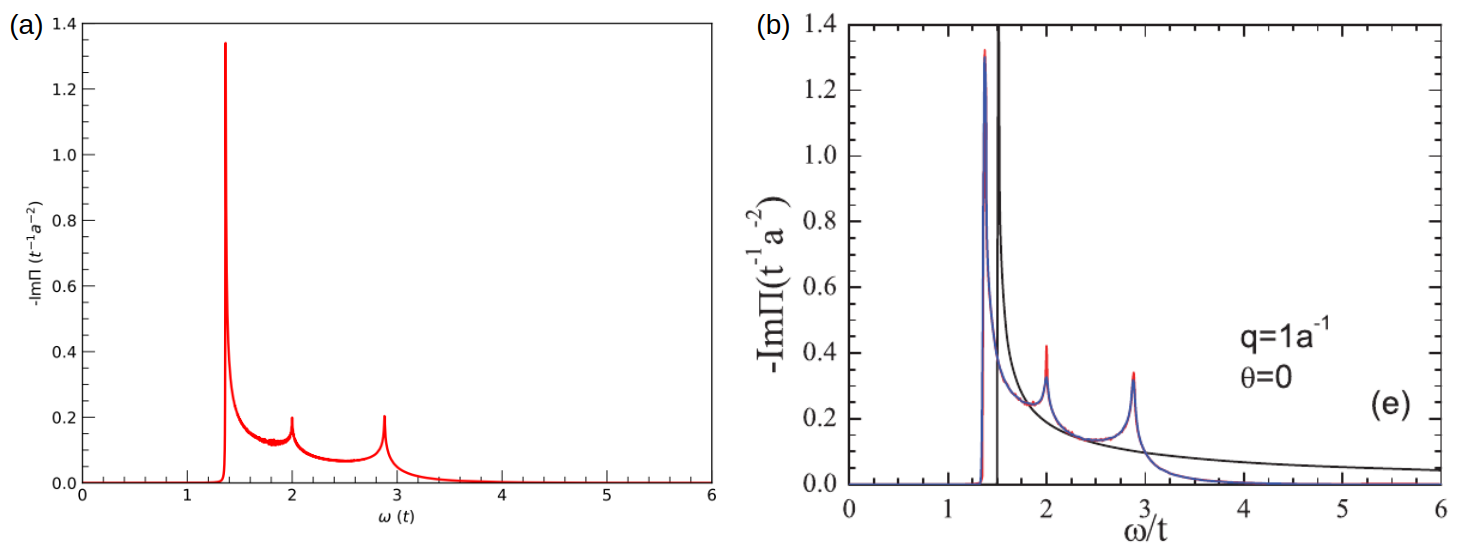
Dynamic polarization of monolayer graphene for \(|q| = 1/a\) and \(\theta = 30^\circ\). (a) Output of this tutorial. (b) Fig. 3(e) of Phys. Rev. B 84, 035439 (2011).

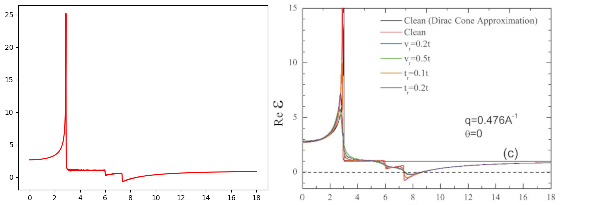
Dielectric function of \(|q|=4.76 nm^{-1}\) and \(\theta = 30^\circ\). (a) Output of this tutorial. (b) Fig. 7(c) of Phys. Rev. B 84, 035439 (2011).

AC conductivity

AC conductivity can be evaluate in a similar approach to dynamic polarization:

def calc_ac_cond() -> None:
    """
    Calculate ac conductivity of monolayer graphene.
    """
    # Model parameters
    # t: hopping integral in eV
    t = 3.0

    # Create model, solver and set parameters
    cell = tb.make_graphene_diamond(t=t)
    lind = tb.Lindhard(cell)
    lind.config.prefix = "ac_cond"
    lind.config.e_min = 0.0
    lind.config.e_max = 18.0
    lind.config.e_step = 0.005
    lind.config.dimension = 2
    lind.config.num_spin = 2
    lind.config.k_grid_size = (2048, 2048, 1)
    omegas, ac_cond = lind.calc_ac_cond()

    # Plot
    plot_ac_cond(omegas, ac_cond, t=t)

We also need to create the model, the solver and set up parameters. Most of the parameters are the same to dynamic polarization. To be consistent with Phys. Rev. B 82, 115448 (2010), we use a k-grid of \(2048 \times 2048 \times 1\), and set the spin-degeneracy to 2 via the num_spin parameter. Other parameters not shown in the example include ac_cond_component which defines the component of ac conductivity to evaluate. The AC conductivity can be obtained by calling the calc_ac_cond method. The function to visualize the results is defined as:

def plot_ac_cond(omegas: np.ndarray,
                 ac_cond: np.ndarray,
                 t: float = 3.0) -> None:
    """
    Plot ac conductivity.
    :param omegas: (num_eng,) float64 array, energy grid in eV
    :param ac_cond: (num_eng,) complex128 array, ac conductivity
    :param t: hopping integral in eV
    :return: None
    """
    # Reference: fig. 13 of [2]
    plt.plot(omegas / t, ac_cond.real * 4, color="red")
    plt.xticks(np.linspace(0.0, 6.0, 7))
    plt.yticks(np.linspace(0.0, 4.0, 9))
    plt.xlim(0.0, 6.0)
    plt.ylim(0.0, 4.0)
    plt.minorticks_on()
    plt.tick_params(which="major", direction="out", length=8, width=0.6)
    plt.tick_params(which="minor", direction="out", length=4, width=0.6)
    plt.xlabel(r"$\omega\ (t)$")
    plt.ylabel(r"$\sigma_{xx}\ (\sigma_0)$")
    plt.tight_layout()
    plt.savefig("ac_cond.pdf")
    plt.close()

The result is shown in Fig.3:

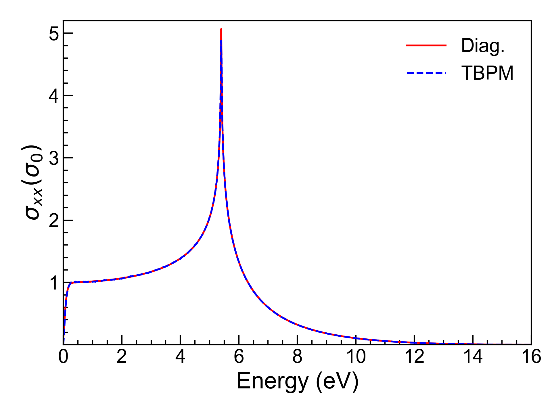
AC conductivity of monolayer graphene. (a) Output of this tutorial. (b) Fig. 3(e) of Phys. Rev. B 82, 115448 (2010).

Notes on system dimension

The formulae for calculating dynamic polarization, dielectric function and AC conductivity are defines as:

\[\Pi(\textbf{q},\omega)=\frac{g_s}{(2\pi)^n}\int_{\mathrm{BZ}}\mathrm{d}^n\textbf{k}\sum_{l,l^\prime}\frac{n_\mathrm{F}(E_{\textbf{k}l})-n_\mathrm{F}(E_{\textbf{k}^{\prime}l^{\prime}})}{E_{\textbf{k}l}-E_{\textbf{k}^{\prime}l^{\prime}}+\hbar\omega+\mathrm{i}\eta^+}|\langle\textbf{k}^{\prime}l^{\prime}|\mathrm{e^{\mathrm{i}\textbf{q}\cdot\textbf{r}}|\textbf{k}l\rangle}|^2\]

\[\epsilon(\textbf{q},\omega)=1-V(\textbf{q})\Pi(\textbf{q},\omega)\]

\[\sigma_{\alpha\beta}(\omega)=\frac{\mathrm{i} e^2 \hbar}{N_k \Omega_c}\sum_{\textbf k}\sum_{n,m} \frac{f_{m\textbf{k}} - f_{n\textbf{k}}}{\epsilon_{m\textbf{k}} - \epsilon_{n\textbf{k}}} \frac{\langle\psi_{n\textbf k}|v_\alpha|\psi_{m\textbf k}\rangle \langle\psi_{m\textbf k}|v_\beta|\psi_{n\textbf k}\rangle}{\epsilon_{m\textbf{k}} - \epsilon_{n\textbf{k}}-(\hbar\omega+\mathrm i\eta^+)}\]

Lindhard class deals with system dimension in two approaches. The first approach is to treat all systems as 3-dimensional. In this approach, supercell technique is required, with vacuum layers added on non-periodic directions. Also, the component(s) of k_grid_size should be set to 1 accordingly on that direction. The seond approach utilizes dimension-specific formula whenever possible. For now, only 2-dimensional case has been implemented. This approach requires that the system should be periodic in \(xOy`\) plane, i.e. the non-periodic direction should be along \(c\) axis.

Regarding the accuracy of results, the first approach suffers from the issue that dynamic polarization and AC conductivity scale inversely proportional to the product of supercell lengths, i.e., \(|c|\) in 2d case and \(|a|*|b|\) in 1d case. This is caused by elementary volume in reciprocal space (\(\mathrm{d}^{3}k\)) in Lindhard function. On the contrary, the second approach has no such issue. If the supercell lengths of non-periodic directions are set to 1 nm, then the first approach yields the same results as the second approach.

For the dielectric function, the situation is more complicated. From the equation for epsilon we can see that it is also affected by the Coulomb potential \(V(q)\), which is \(V(q)=\frac{1}{\epsilon_0\epsilon_r}\cdot\frac{4\pi e^2}{q^2}\) in 3-d case and \(V(q)=\frac{1}{\epsilon_0\epsilon_r}\cdot\frac{2\pi e^2}{q}\) in 2-d case, respectively. So the influence of system dimension is q-dependent. Setting supercell length to 1 nm will NOT reproduce the same result as the second approach.