Chern number and Berry curvature
In this tutorial, we demonstrate the usage of Berry class by calculating the Chern number
and Berry curvature of Haldane model. The corresponding script is located at examples/prim_cell/berry.py.
We begin with importing the necessary packages:
import numpy as np

import tbplas as tb
and define the function for generating the Haldane model:
 1def make_haldane() -> tb.PrimitiveCell:
 2    """
 3    Make Haldane model for testing Berry utilities.
 4    Reference: examples/haldane.py of pythtb
 5    """
 6    lat = 1.0
 7    delta = 0.2
 8    t = -1.0
 9    t2 = 0.15 * np.exp(1j * np.pi / 2.)
10    t2c = t2.conjugate()
11
12    vectors = tb.gen_lattice_vectors(a=lat, b=lat, c=1.0, gamma=60)
13    cell = tb.PrimitiveCell(vectors, unit=tb.NM)
14    cell.add_orbital((1 / 3., 1 / 3.), energy=-delta)
15    cell.add_orbital((2 / 3., 2 / 3.), energy=delta)
16    cell.add_hopping((0, 0), 0, 1, t)
17    cell.add_hopping((1, 0), 1, 0, t)
18    cell.add_hopping((0, 1), 1, 0, t)
19    cell.add_hopping((1, 0), 0, 0, t2)
20    cell.add_hopping((1, -1), 1, 1, t2)
21    cell.add_hopping((0, 1), 1, 1, t2)
22    cell.add_hopping((1, 0), 1, 1, t2c)
23    cell.add_hopping((1, -1), 0, 0, t2c)
24    cell.add_hopping((0, 1), 0, 0, t2c)
25    return cell
Chern number
We define the following function to demonstrate the calculation of Chern number:
 1def calc_chern_number() -> None:
 2    """Calculate Chern number of Haldane model."""
 3    # Create model and solver.
 4    cell = make_haldane()
 5    solver = tb.Berry(cell)
 6
 7    # Set up parameters
 8    solver.config.k_grid_size = (100, 100, 1)
 9    solver.config.num_occ = 1
10
11    # Calculate Berry curvature and Chern number using Kubo formula
12    solver.config.prefix = "chern_kubo"
13    solver.calc_berry_curvature_kubo()
14
15    # Calculate Berry curvature and Chern number using Wilson loop
16    solver.config.prefix = "chern_wilson"
17    solver.calc_berry_curvature_wilson()
Just as in other tutorials, we firstly create the model and the solver, then set up the calculation
parameters. We need to sample the first Brillouin zone (FBZ) with k-grid specified by k_grid_size,
and the number of occupied states by num_occ. Then we call calc_berry_curvature_kubo and
calc_berry_curvature_wilson to calculate the Berry curvature and Chern number using Kubo formula
and Wilson loop methods, respectively. The output should look like:
1... ...
2Chern number for band 0: -1
3Chern number for band 1: 1
4
5... ...
6Chern number for num_occ 1: -1
indicating the Chern number for the two bands is -1 and 1, respectively. The total Chern number is -1, since there is only one occupied band.
Berry curvature
The calc_berry_curvature_kubo and calc_berry_curvature_wilson methods already output the
Berry curvatures in FBZ. For better appearance, we need to extend k-grid to second Brillouin zone.
This is done by the bz_size parameter, as demonstrated in the following function:
 1def calc_berry_curvature() -> None:
 2    """Calculate and visualize Berry curvature of Haldane model."""
 3    # Create model and solver.
 4    cell = make_haldane()
 5    solver = tb.Berry(cell)
 6
 7    # Set up parameters
 8    solver.config.k_grid_size = (100, 100, 1)
 9    solver.config.bz_size = (2, 2, 1)
10    solver.config.num_occ = 1
11
12    # Calculate Berry curvature and Chern number using Kubo formula
13    solver.config.prefix = "berry_kubo"
14    data_kubo = solver.calc_berry_curvature_kubo()
15
16    # Calculate Berry curvature and Chern number using Wilson loop
17    solver.config.prefix = "berry_wilson"
18    data_wilson = solver.calc_berry_curvature_wilson()
19
20    # Visualization
21    if solver.is_master:
22        plot_omega_xy(data_kubo, ib=0)
23        plot_omega_xy(data_kubo, ib=1)
24        plot_omega_xy(data_wilson)
The functions for visualizing Berry curvature is defined as:
 1def plot_omega_xy(berry_data: tb.BerryData, ib: int = 0) -> None:
 2    """
 3    Visualize Berry curvature.
 4    :param berry_data: Berry curvature to plot
 5    :param ib: band index of Berry curvature to plot
 6    :return: None
 7    """
 8    kpt_cart = berry_data.kpt_cart
 9    omega_xy = berry_data.omega_xy[:, ib]
10    vis = tb.Visualizer()
11    vis.plot_scalar(x=kpt_cart[:, 0], y=kpt_cart[:, 1], z=omega_xy, scatter=True,
12                    num_grid=(480, 480), cmap="jet", with_colorbar=True)
The output is shown the figure below:
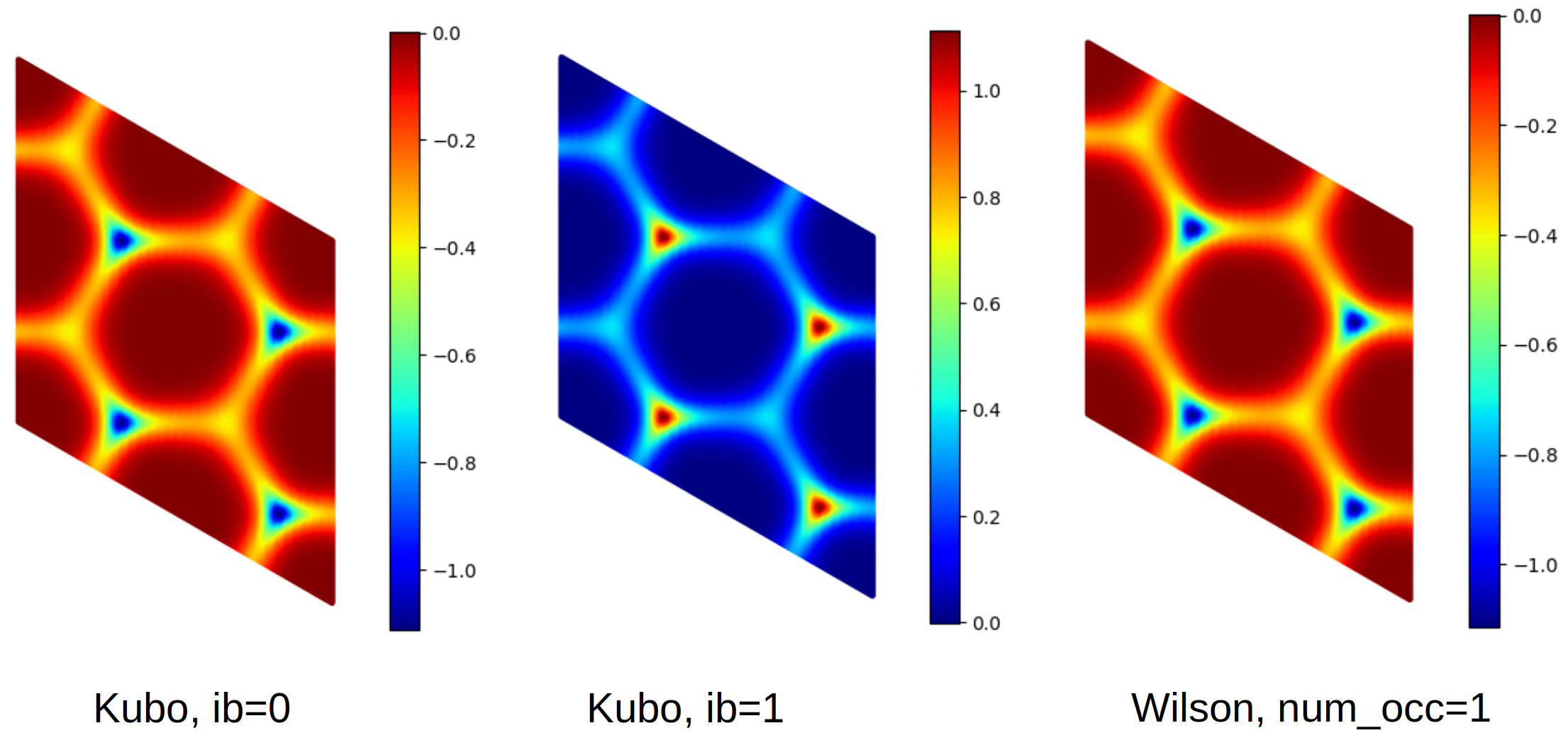
Berry curvatures from Kubo formula and Wilson loop methods.