Parameters fitting

In this tutorial, we show how to fit the on-site energies and hopping terms by reducing the 8-band graphene primitive cell imported from the output of Wannier90 in Interfaces. We achieve this by truncating the hopping terms to the second nearest neighbor, and refitting the on-site energies and Slater-Koster parameters to minimize the residual between the reference and fitted band data, i.e.

\[\min_{\mathbf{x}} \sum_{i,\mathbf{k}}\omega_i\left|\bar{E}_{i,\mathbf{k}} - E_{i,\mathbf{k}}(\mathbf{x})\right|^2\]

where \(\mathbf{x}\) are the fitting parameters, \(\omega\) are the fitting weights, \(\bar{E}\) and \(E\) are the reference and fitted band data from the original and reduced cells, \(i\) and \(\mathbf{k}`\) are band and \(\mathbf{k}\)-point indices, respectively. The corresponding script can be found at examples/interface/wannier90/graphene/fit.py. We begin with importing the necessary packages:

import numpy as np
import matplotlib.pyplot as plt

import tbplas as tb

Auxialiary functions and classes

We define the following functions to build the primitive cell from the Slater-Koster paramaters. Most of them are similar to the functions in Slater-Koster formulation:

def calc_hop(sk: tb.SK, rij: np.ndarray, distance: float,
             label_i: str, label_j: str, sk_params: np.ndarray) -> complex:
    """
    Calculate hopping integral based on Slater-Koster formulation.

    :param sk: SK instance
    :param rij: displacement vector from orbital i to j in nm
    :param distance: norm of rij
    :param label_i: label of orbital i
    :param label_j: label of orbital j
    :param sk_params: array containing SK parameters
    :return: hopping integral in eV
    """
    # 1st and 2nd hopping distances in nm
    d1 = 0.1419170044439990
    d2 = 0.2458074906840380
    if abs(distance - d1) < 1.0e-5:
        v_sss, v_sps, v_pps, v_ppp = sk_params[2:6]
    elif abs(distance - d2) < 1.0e-5:
        v_sss, v_sps, v_pps, v_ppp = sk_params[6:10]
    else:
        raise ValueError(f"Too large distance {distance}")
    return sk.eval(r=rij, label_i=label_i, label_j=label_j,
                   v_sss=v_sss, v_sps=v_sps,
                   v_pps=v_pps, v_ppp=v_ppp)


def make_cell(sk_params: np.ndarray) -> tb.PrimitiveCell:
    """
    Make primitive cell from Slater-Koster parameters.

    :param sk_params: (10,) float64 array containing Slater-Koster parameters
    :return: created primitive cell
    """
    # Lattice constants and orbital info.
    lat_vec = np.array([
        [2.458075766398899, 0.000000000000000, 0.000000000000000],
        [-1.229037883199450, 2.128755065595607, 0.000000000000000],
        [0.000000000000000, 0.000000000000000, 15.000014072326660],
    ])
    orb_pos = np.array([
        [0.000000000, 0.000000000, 0.000000000],
        [0.666666667, 0.333333333, 0.000000000],
    ])
    orb_label = ("s", "px", "py", "pz")

    # Create the cell and add orbitals
    e_s, e_p = sk_params[0], sk_params[1]
    cell = tb.PrimitiveCell(lat_vec, unit=tb.ANG)
    for pos in orb_pos:
        for label in orb_label:
            if label == "s":
                cell.add_orbital(pos, energy=e_s, label=label)
            else:
                cell.add_orbital(pos, energy=e_p, label=label)

    # Add Hopping terms
    neighbors = tb.find_neighbors(cell, a_max=5, b_max=5,
                                  max_distance=0.25)
    sk = tb.SK()
    for term in neighbors:
        i, j = term.pair
        label_i = cell.get_orbital(i).label
        label_j = cell.get_orbital(j).label
        hop = calc_hop(sk, term.rij, term.distance, label_i, label_j,
                       sk_params)
        cell.add_hopping(term.rn, i, j, hop)
    return cell

The fitting tool ParamFit is an abstract class. The users should derive their own fitting class from it, and implement the calc_bands_ref and calc_bands_fit methods, which return the reference and fitted band data, respectively. We define a MyFit class as

class MyFit(tb.ParamFit):
    def calc_bands_ref(self) -> np.ndarray:
        """
        Get reference band data for fitting.

        :return: band structure on self._k_points
        """
        cell = tb.wan2pc("graphene")
        k_len, bands = cell.calc_bands(self._k_points)
        return bands

    def calc_bands_fit(self, sk_params: np.ndarray) -> np.ndarray:
        """
        Get band data of the model from given parameters.

        :param sk_params: array containing SK parameters
        :return: band structure on self._k_points
        """
        cell = make_cell(sk_params)
        k_len, bands = cell.calc_bands(self._k_points, echo_details=False)
        return bands

In calc_bands_ref, we import the primitive cell with the Wannier90 interface wan2pc(), then calculate and return the band data. The calc_bands_fit function does a similar job, with the only difference that the primitive cell is constructed from Slater-Koster parameters with the make_cell function we have just created.

Fitting the paramaters

The application of MyFit class is as following:

def main():
    # Fit the sk parameters
    # Reference:
    # https://journals.aps.org/prb/abstract/10.1103/PhysRevB.82.245412
    k_points = tb.gen_kmesh((120, 120, 1))
    weights = np.array([1.0, 1.0, 1.0, 1.0, 1.0, 1.0, 1.0, 1.0])
    fit = MyFit(k_points, weights)
    sk0 = np.array([-8.370, 0.0,
                    -5.729, 5.618, 6.050, -3.070,
                    0.102, -0.171, -0.377, 0.070])
    sk1 = fit.fit(sk0)
    print("SK parameters after fitting:")
    print(sk1[:2])
    print(sk1[2:6])
    print(sk1[6:10])

    # Plot fitted band structure
    k_points = np.array([
        [0.0, 0.0, 0.0],
        [1./3, 1./3, 0.0],
        [1./2, 0.0, 0.0],
        [0.0, 0.0, 0.0],
    ])
    k_path, k_idx = tb.gen_kpath(k_points, [40, 40, 40])
    cell_ref = tb.wan2pc("graphene")
    cell_fit = make_cell(sk1)
    k_len, bands_ref = cell_ref.calc_bands(k_path)
    k_len, bands_fit = cell_fit.calc_bands(k_path)
    num_bands = bands_ref.shape[1]
    for i in range(num_bands):
        plt.plot(k_len, bands_ref[:, i], color="red", linewidth=1.0)
        plt.plot(k_len, bands_fit[:, i], color="blue", linewidth=1.0)
    plt.show()


if __name__ == "__main__":
    main()

To create a MyFit instance, we need to specify the \(\mathbf{k}\)-points and fitting weights, as shown in line 5-6. For the \(\mathbf{k}\)-points, we are going to use a \(\mathbf{k}\)-grid of \(120\times120\times1\). The length of weights should be equal to the number of orbitals of the primitive cell, which is 8 in our case. We assume all the bands to have the same weights, and set them to 1. Then we create the MyFit instance, define the initial guess of parameters from the reference, and get the fitted results with the fit function. The output should look like

SK parameters after fitting:
[-3.63102899 -1.08477167]
[-5.27742318  5.87219052  4.61650991 -2.75652966]
[-0.24734558  0.17599166  0.14798703  0.16545428]

The first two numbers are the on-site energies for \(s\) and \(p\) orbitals, while the following numbers are the Slater-Koster paramets \(V_{ss\sigma}\), \(V_{sp\sigma}\), \(V_{pp\sigma}\) and \(V_{pp\pi}`\) at first and second nearest hopping distances, respectively. We can also plot and compare the band structures from the reference and fitted primitive cells, as shown the left panel of the figure. It is clear that the fitted band structure agrees well with the reference data near the Fermi level (-1.7 eV) and at deep (-20 eV) or high energies (10 eV). However, the derivation from reference data of intermediate bands (-5 eV and 5 eV) is non-negligible. To improve this, we lower the weights of band 1-2 and 7-8 by

weights = np.array([0.1, 0.1, 1.0, 1.0, 1.0, 1.0, 0.1, 0.1])

and refitting the parameters. The results are shown in the right panel of the figure, where the fitted and reference band structures agree well from -5 to 5 eV.

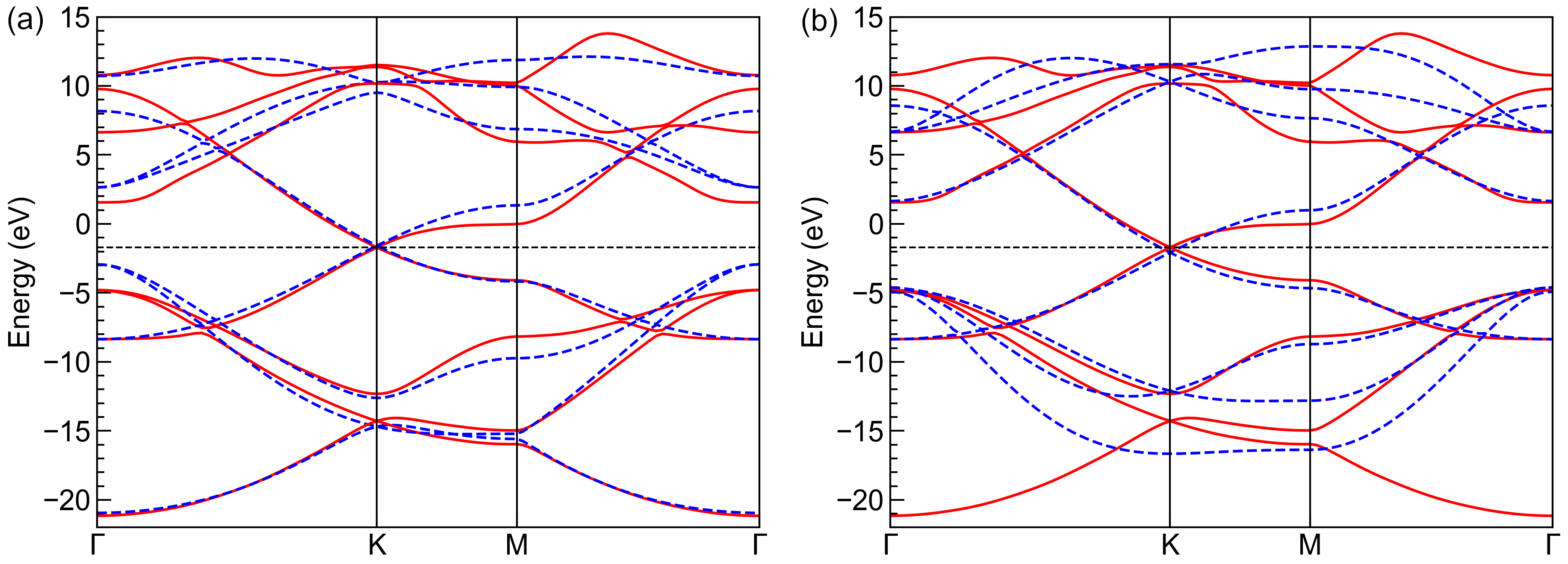
Band structures from reference (solid red lines) and fitted (dashed blue lines) primitive cells with (a) equal weights for all bands and (b) lower weights for bands 1-2 and 7-8. The horizontal dashed black lines indicate the Fermi level.