Properties from TBPM

In this tutorial, we demonstrate the usage of Tight-Binding Propagation Methods (TBPM) implemented in TBPLaS, by calculating the DOS and AC conductivity of monolayer graphene. TBPM can solve a lot of electronic and response properties of large tight-binding models in a much faster way than exact diagonalization. For the capabilities of TBPM, see Features.

In general, all TBPM calculations begin with setting up a sample from the Sample class and a solver from the TBPMSolver class taking the sample as argument. Then the calculation parameters are set by modifying the config attribute of the solver, which is an instance of the TBPMConfig class. Afterwards, the solver is utilized to evaluate correlation functions, which are then post-processed to yield desired properties. The analyzer is created from the Analyzer class. Finally, the results are visualized by a visualizer of the Visualizer class or by matplotlib directly.

The example script can be found at examples/sample/tbpm/graphene.py, while the full capabilities of TBPM is demonstrated in tbplas-cpp/samples/speedtest/tbpm.py. We begin with importing the necessary packages:

import numpy as np
import matplotlib.pyplot as plt

import tbplas as tb

DOS

TBPM requires a large model for better convergence. So we firstly create a graphene sample with \(1024 \times 1024 \times 1\) cells:

prim_cell = tb.make_graphene_diamond()
super_cell_pbc = tb.SuperCell(prim_cell, dim=(1024, 1024, 1),
                              pbc=(True, True, True))
sample_pbc = tb.Sample(super_cell_pbc)

Then we create the solver and analyzer:

solver = tb.TBPMSolver(sample_pbc)
analyzer = tb.Analyzer(f"{solver.config.prefix}_info.dat")

And set up the calculation parameters:

solver.config.rescale = 9.0
solver.config.num_random_samples = 1
solver.config.num_time_steps = 1024

The propagation of wave function is simulated with the algorithm of Chebyshev decomposition of Hamiltonian, which requires the eigenvalues of Hamiltonian to be on the range of \([-1, 1]\). So we need to set the rescaling factor of Hamiltonian by the rescale argument. If not set, the scaling factor will be estimated by inspecting the Hamiltonian automatically. The number of random initial conditions is given by num_random_samples and the number of propagation steps is given by num_time_steps. After setting the parameters, we evaluate and analyze the correlation function:

tbpm_dos(solver, analyzer)

which is defined as:

def tbpm_dos(solver: tb.TBPMSolver, analyzer: tb.Analyzer) -> None:
    """
    Calculate DOS with TBPM.

    :param solver: TBPM solver
    :param analyzer: TBPM analyzer
    :return: None
    """
    # Get DOS correlation function with solver.
    corr_dos = solver.calc_corr_dos()

    # Analyze DOS correlation function with analyzer.
    energies_dos, dos = analyzer.calc_dos(corr_dos)

    # Plot DOS
    plt.plot(energies_dos, dos)
    plt.xlabel("Energy (eV)")
    plt.ylabel("DOS")
    plt.savefig("DOS.png")
    plt.close()

The output is shown in panel (a) of the figure:

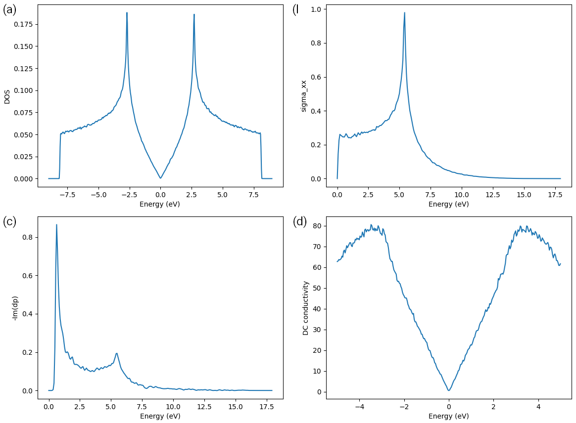
../../_images/tbpm.png — Density of states (a), optical (AC) conductivity (b) conductivity (d) of graphene sample.

AC conductivity

We then demonstrate more capabilities of TBPM. Firstly, we set the spin-degeneracy to 2:

solver.config.num_spin = 2

Then evaluate AC conductivity in a similar approach as DOS:

tbpm_ac_cond(solver, analyzer)

The tbpm_ac_cond function is defined as:

def tbpm_ac_cond(solver: tb.TBPMSolver, analyzer: tb.Analyzer) -> None:
    """
    Calculate AC conductivity with TBPM.

    :param solver: TBPM solver
    :param analyzer: TBPM analyzer
    :return: None
    """
    corr_ac = solver.calc_corr_ac_cond()
    omegas_ac, ac = analyzer.calc_ac_cond(corr_ac)
    plt.plot(omegas_ac, ac[0].real)
    plt.xlabel("Energy (eV)")
    plt.ylabel("sigma_xx")
    plt.savefig("ACxx.png")
    plt.close()

The results are shown in panel (b) of the figure.

Convergence

We do not perform convergence tests in the examples for saving time. In actual calculations, convergence should be checked with respect to sample size, number of initial conditions and propagation steps, etc.

If the primitive cell is large enough, then reduce the dim argument when creating the supercell accordingly. Taking twisted bilayer graphene as example, for \(\theta=1.05^\circ\) there are 11,908 orbitals in a primitive cell, then dim=(10, 10, 1) is almost enough for convergence. If the primitive cell contains millions of orbitals (honestly, it is beyond the capability of the Python PrimitiveCell class), then dim=(1, 1, 1) is enough. But the SuperCell class does not allow such dim by default. In that case, add the check_dim=False argument to skip the dimension check when constructing the supercell.