Strain and external fields

In this tutorial, we introduce the common procedure of applying strain and external fields on the model. It is difficult to design common out-of-the-box user APIs that offer such functionalities since they are strongly case-dependent. Generally, the user should implement these perturbations by modifying model attributes such as orbital positions, on-site energies and hopping integrals. For the primitive cell, it is straightforward to achieve this goal with the set_orbital and add_hopping methods. The Sample class, on the contrary, does not offer such methods. Instead, the user should work with the attributes directly. In the Sample class, orbital positions and on-site energies are stored in the orb_pos and orb_eng attributes. Hopping terms are represented with 2 attributes: hop_ind for orbital indices, and hop_eng for hopping integrals. There is also an auxiliary attribute dr which holds the hopping vectors. All the attributes are NumPy arrays. The on-site energies and hopping terms can be modified directly, while the orbital positions should be changed via a modifier function. The hopping vectors are updated from the orbital positions and hopping terms automatically, thus no need of explicit modification.

As the example, we will investigate the propagation of wave function in a graphene sample. The script can be found at examples/advanced/strain_fields.py. We begin with defining the functions for adding strain and external fields, then calculate and plot the time-dependent wave function to check their effects on the propagation. The essential packages of this tutorial can be imported with:

import math
from typing import Callable, Tuple

import numpy as np
from numpy.linalg import norm

import tbplas as tb

Functions for strain

Strain will introduce deformation into the model, changing both orbital positions and hopping integrals. It is a rule that orbital positions should not be modified directly, but through a modifier function. We consider a Gaussian bump deformation, and define the following functions to generate the modifier:

def gaussian(orb_pos: np.ndarray,
             center: np.ndarray,
             sigma: Tuple[float, float] = (0.5, 0.5),
             extent: Tuple[float, float] = (1.0, 1.0)) -> Dict[str, np.ndarray]:
    """
    Generate normalized Gaussian distribution based on the orbital positions.

    :param orb_pos: (num_orb, 3) float64 array, orbital positions in nm
    :param center: Cartesian coordinate of the Gaussian center in nm
    :param sigma: width of Gaussian along x and y directions in nm
    :param extent: factors controlling Gaussian extent along x and y directions
    :return: the Gaussian distribution
    """
    dx = (orb_pos[:, 0] - center[0]) * extent[0]
    dy = (orb_pos[:, 1] - center[1]) * extent[1]
    amp = np.exp(- dx ** 2 / (2 * sigma[0] ** 2) - dy ** 2 / (2 * sigma[1] ** 2))
    amp /= (2 * math.pi * np.prod(sigma))
    result = {"dx": dx, "dy": dy, "amp": amp}
    return result


def make_deform(scale: Tuple[float, float] = (0.5, 0.5), **kwargs) -> Callable:
    """
    Generate Gaussian-shaped deformation function as orb_pos_modifier.

    :param scale: scaling factors for deformation along xOy and z directions
    :param kwargs: arguments for 'gaussian' function
    :return: deformation function
    """
    def _deform(orb_pos):
        g = gaussian(orb_pos, **kwargs)
        orb_pos[:, 0] += g["dx"] * g["amp"] * scale[0]
        orb_pos[:, 1] += g["dy"] * g["amp"] * scale[0]
        orb_pos[:, 2] += g["amp"] * scale[1]
    return _deform

The arguments center, sigma and extent in function gaussian control the location, width and extent of the Gaussian distribution, respectively. For example, if extent is set to \((1.0, 0.0)\), the distribution will become one-dimensional which varies along \(x\)-direction while remains constant along \(y\)-direction. The scale argument in function make_deform specifies the scaling factors for in-plane and out-of-plane displacements. The make_deform function returns another function as the modifier, which updates the orbital positions in place according to the following expression:

\[\begin{split}\mathbf r_i &\rightarrow \mathbf r_i + \Delta_i \\ \Delta_i^{\parallel} &= A_i \cdot (\mathbf r_i^{\parallel} - \mathbf c_0^{\parallel}) \cdot s^{\parallel} \\ \Delta_i^{\perp} &= A_i \cdot s^{\perp} \\ A_i &= \exp \left[-\frac{1}{2\sigma^2}\sum_{j=1}^{2} (\mathbf r_i^j - \mathbf c_0^j)^2 \cdot \eta^j \right]\end{split}\]

where \(\mathbf{r}_i\) is the position of \(i\)-th orbital, \(\Delta_i\) is the displacement, \(s\) is the scaling factor, \(\parallel\) and \(\perp\) are the in-plane and out-of-plane components. The location, width and extent of the Gaussian bump are denoted as \(\mathbf{c}_0\), \(\sigma\) and \(\eta\), respectively.

In addition to the orbital position modifier, we also need to update hopping integrals

def update_hop(sample: tb.Sample) -> None:
    """
    Update hopping terms in presence of deformation.

    :param sample: Sample to modify
    :return: None.
    """
    sample.init_hop()
    for i, rij in enumerate(sample.dr):
        sample.hop_eng[i] = calc_hop(rij)

As we will make use of the hopping terms and vectors, we should call the init_hop method to initialize the attributes. Similar rule holds for the on-site energies and orbital positions. Then we loop over the hopping terms to update the integrals in hop_eng according to the vectors in dr with the calc_hop function, which is defined as:

def calc_hop(rij: np.ndarray) -> float:
    """
    Calculate hopping parameter according to Slater-Koster relation.
    See ref. [2] for the formulae.

    :param rij: (3,) array, displacement vector between two orbitals in NM
    :return: hopping parameter in eV
    """
    a0 = 0.1418
    a1 = 0.3349
    r_c = 0.6140
    l_c = 0.0265
    gamma0 = 2.7
    gamma1 = 0.48
    decay = 22.18
    q_pi = decay * a0
    q_sigma = decay * a1
    dr = norm(rij).item()
    n = rij.item(2) / dr
    v_pp_pi = - gamma0 * math.exp(q_pi * (1 - dr / a0))
    v_pp_sigma = gamma1 * math.exp(q_sigma * (1 - dr / a1))
    fc = 1 / (1 + math.exp((dr - r_c) / l_c))
    hop = (n**2 * v_pp_sigma + (1 - n**2) * v_pp_pi) * fc
    return hop

Functions for external fields

The effects of external electric field can be modeled by adding position-dependent potential to the on-site energies. We consider a Gaussian-type scattering potential described by

\[V_i = V_0 \cdot A_i\]

and define the following function to add the potential to the sample

def add_efield(sample: tb.Sample, v_pot: float = 1.0, **kwargs) -> None:
    """
    Add Gaussian-shaped electric field to the sample.

    :param sample: sample to add the field
    :param v_pot: electric field intensity in eV
    :param kwargs: arguments for 'gaussian'
    :return: None.
    """
    sample.init_orb_pos()
    sample.init_orb_eng()
    sample.orb_eng += v_pot * gaussian(sample.orb_pos, **kwargs)["amp"]

The argument v_pot specifies \(V_0\). Similar to update_hop, we need to call init_orb_pos and init_orb_eng to initialize orbital positions and on-site energies before accessing them. Then the position-dependent scattering potential is added to the on-site energies.

The effects of magnetic field can be modeled with Peierls substitution. For homogeneous magnetic field perpendicular to the \(xOy\)-plane along \(-z\) direction, the Sample class offers an API apply_magnetic_field, which follows the Landau gauge of vector potential \(\mathbf{A} = (By, 0, 0)\) and updates the hopping terms as

\[t_{ij} \rightarrow t_{ij} \cdot \exp \left[\mathrm i\frac{eB}{2\hbar c} \cdot (\mathbf r_j^x - \mathbf r_i^x) \cdot (\mathbf r_j^y + \mathbf r_i^y) \right]\]

where \(B\) is the intensity of magnetic field, \(\mathbf{r}_i\) and \(\mathbf{r}_j\) are the positions of \(i\)-th and \(j\)-th orbitals, respectively.

Initial wave functions

The initial wave function we consider here as an example for the propagation is a Gaussian wave-packet, which is defined by

def init_wfc_gaussian(sample: tb.Sample, **kwargs) -> np.ndarray:
    """
    Generate Gaussian wave packet as initial wave function.

    :param sample: sample for which the wave function shall be generated
    :param kwargs: arguments for 'gaussian'
    :return: initial wave function
    """
    sample.init_orb_pos()
    wfc = np.array(gaussian(sample.orb_pos, **kwargs)["amp"], dtype=np.complex128)
    wfc /= np.linalg.norm(wfc)
    return wfc

Note that the wave function should be a complex vector whose length must be equal to the number of orbitals. Also, it should be normalized before being returned.

Propagation of wave function

We consider a rectangular graphene sample with \(50\times20\times1\) primitive cells, as shown in Fig. 1(a). We begin with defining some geometric parameters:

prim_cell = tb.make_graphene_rect()
dim = (50, 20, 1)
pbc = (True, True, False)
x_max = prim_cell.lat_vec[0, 0] * dim[0]
y_max = prim_cell.lat_vec[1, 1] * dim[1]
wfc_center = (x_max * 0.5, y_max * 0.5)
deform_center = (x_max * 0.75, y_max * 0.5)

Here dim and pbc define the dimension and boundary condition. x_max and y_max are the lengths of the sample along \(x\) and \(y\) directions. The initial wave function will be a Gaussian wave-packet located at the center of the sample given by wfc_center. The deformation and scattering potential will be located at the center of right half of the sample, as specified by deform_center and shown in Fig. 1(b)-(c).

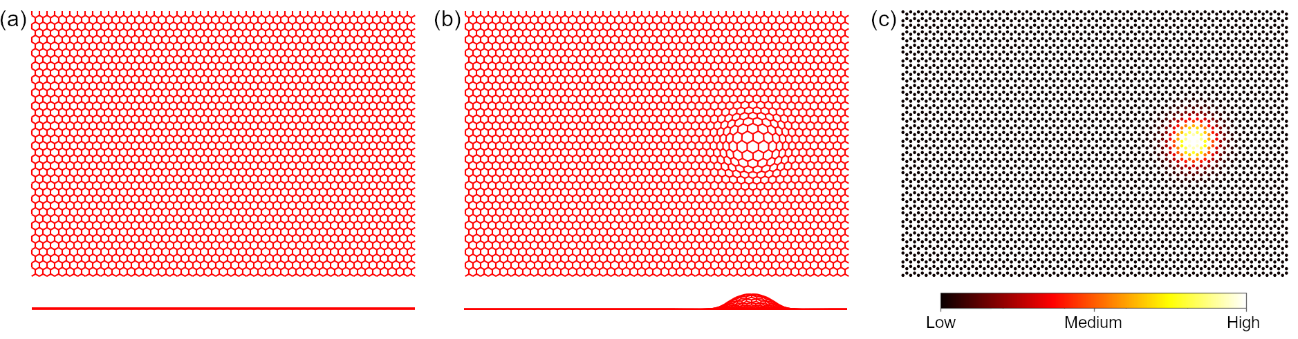
Top and side views of (a) pristine graphene sample and (b) sample with deformation. (c) Plot of on-site energies of graphene sample with scattering potential.

We firstly investigate the propagation of a one-dimensional Gaussian wave-packet in pristine sample, which is given by

# Prepare the sample and inital wave function
sample = tb.Sample(tb.SuperCell(prim_cell, dim, pbc))
psi0 = init_wfc_gaussian(sample, center=wfc_center, extent=(1.0, 0.0))

# Propagate the wave function
time_log = np.array([0, 16, 32, 64, 128])
solver = tb.TBPMSolver(sample)
solver.config.rescale = 10.0
solver.config.num_time_steps = 128
solver.config.wft_wf0 = psi0
solver.config.wft_time_save = time_log
psi_t = solver.calc_wft()

# Visualize the time-dependent wave function
vis = tb.Visualizer()
for i in range(len(time_log)):
    vis.plot_wfc(sample, np.abs(psi_t[i])**2, cmap="hot", scatter=False)

As the propagation is performed with the calc_wft function of TBPMSolver class, it follows the common procedure of TBPM calculation. We need to set the rescaling factor (rescale), the number of steps of propagation (num_time_steps). The initial state is specified by wft_wf0. We propagate the wave function by 128 steps, and save the snapshots in psi_t at the time steps specified by wft_time_save. The snapshots are then visualized by the plot_wfc function of Visualizer class, as shown in Fig. 2(a)-(e), where the wave-packet diffuses freely, hits the boundary and forms interference pattern.

We then add the bump deformation to the sample, by assigning the modifier function to the supercell and calling update_hop to update the hopping terms

deform = make_deform(center=deform_center)
sample = tb.Sample(tb.SuperCell(prim_cell, dim, pbc, orb_pos_modifier=deform))
update_hop(sample)

The propagation of wave-packet in deformed graphene sample is shown in Fig. 2(f)-(j). Obviously, the wave function gets scattered by the bump. Although similar interference pattern is formed, the propagation in the right part of the sample is significantly hindered, due to the increased inter-atomic distances and reduced hopping integrals at the bump.

Similar phenomena are observed when the scattering potential is added to the sample by

add_efield(sample, center=deform_center)

The time-dependent wave function is shown in Fig. 2(k)-(o). Due to the higher on-site energies, the probability of emergence of electron is suppressed near the scattering center.

As for the effects of magnetic field, it is well known that Landau levels will emerge in the DOS. The analytical solution to Schrodinger’s equation for free electron in homogeneous magnetic field with \(\mathbf{A}=(By, 0, 0)\) shows that the wave function will propagate freely along \(x\) and \(z\)-directions while oscillates along \(y\)-direction. To simulate this process, we apply the magnetic field to the sample by

sample.apply_magnetic_field(50)

The snapshots of time-dependent wave function are shown in Fig. 2(p)-(t). The interference pattern is similar to the case without magnetic field, as the wave function propagates freely along \(x\) direction. However, due to the oscillation along \(y\)-direction, the interference pattern gets distorted during the propagation. These phenomena agree well with the analytical results.

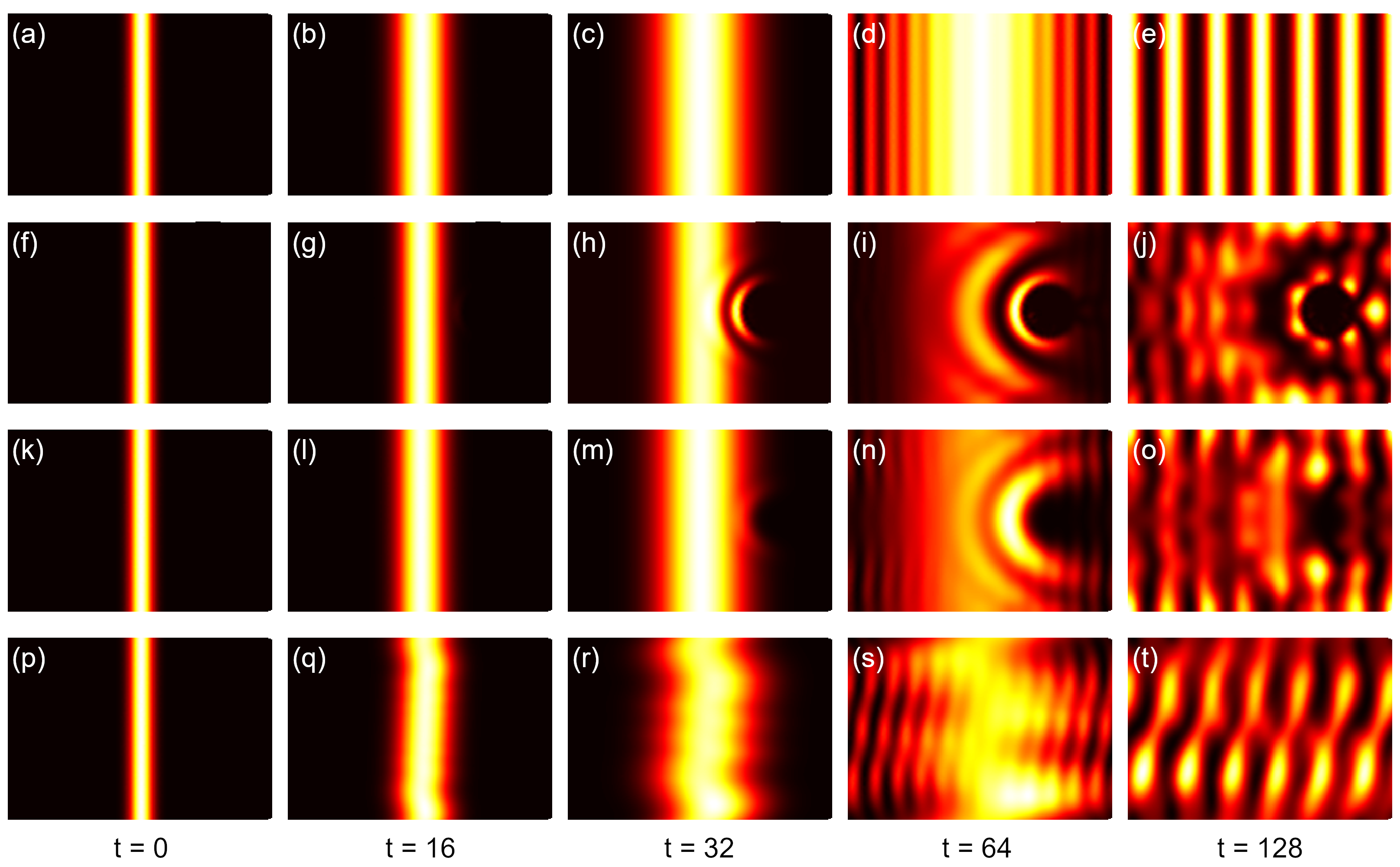
(a)-(e) Propagation of one-dimensional Gaussian wave-packet in pristine graphene sample. (f)-(j) Propagation in graphene sample with deformation, (k)-(o) with scattering potential and (p)-(t) with magnetic field of 50 Tesla.