Non-orthogonal basis set

In this tutorial, we show how to deal with non-orthogonal basis set in diagonalization-based calculations taking monolayer graphene as the example. The script can be found in examples/advanced/non_ortho.py. First of all, we import the necessary packages:

import numpy as np

import tbplas as tb

Then we define the following function to generate the overlap for graphene:

def make_overlap(prim_cell: tb.PrimitiveCell,
                 on_site: float = 1.0,
                 hop: float = 0.0) -> tb.PrimitiveCell:
    """
    Make an overlap for given primitive cell.

    :param prim_cell: primitive cell from which the overlap will be generated
    :param on_site: on-site term of the overlap
    :param hop: hopping terms of the overlap
    :return: overlap with the same numbers of orbitals and hopping terms as the model
    """
    overlap = tb.PrimitiveCell(prim_cell.lat_vec, prim_cell.origin, 1.0)
    for i in range(prim_cell.num_orb):
        orbital = prim_cell.orbitals[i]
        overlap.add_orbital(orbital.position, on_site)

    overlap.add_hopping((0, 0), 0, 1, hop)
    overlap.add_hopping((1, 0), 1, 0, hop)
    overlap.add_hopping((0, 1), 1, 0, hop)
    return overlap

The overlap is actually an instance of the PrimitiveCell class sharing the same lattice vectors, lattice origin and orbital positions. The on-site and hopping terms represent the overlap of the basis functions themselves, and the overlap between different basis functions, respectively. In the orthogonal case, the on-site overlap exactly 1, while the hopping overlap is exactly 0. In the non-orthogonal case, the on-site` overlap is never 1.0, and the hopping overlap is non-zero.

We check the effects of orthogonality of basis functions by calculating the band structure:

def main():
    prim_cell = tb.make_graphene_diamond()
    overlap = make_overlap(prim_cell, on_site=1.0, hop=0.0)
    #overlap = make_overlap(prim_cell, on_site=0.8, hop=0.1)
    solver = tb.DiagSolver(prim_cell, overlap)

    k_points = np.array([
        [0.0, 0.0, 0.0],
        [2./3, 1./3, 0.0],
        [0.5, 0.0, 0.0],
        [0.0, 0.0, 0.0]
    ])
    k_path, k_idx = tb.gen_kpath(k_points, (1000, 1000, 1000))
    solver.config.prefix = "graphene"
    solver.config.k_points = k_path

    timer = tb.Timer()
    timer.tic("bands")
    k_len, bands = solver.calc_bands()
    timer.toc("bands")

    if solver.is_master:
        timer.report_total_time()
        vis = tb.Visualizer()
        vis.plot_bands(k_len, bands, k_idx, ["G", "K", "M", "G"])


if __name__ == "__main__":
    main()

We firstly set on-site to 1.0 and hop to 0.0, i.e., the basis set is orthogonal. Then we set on-site to 0.8 and hop to 0.1 to mimic a non-orthogonal basis set. The overlap instance is passed as the second argument when constructing the solver. Subsequential steps are the same as the orthogonal case. The output is shown in the figure below. It is clear that the non-orthogonal basis set significantly reshapes the band structure, including both the energy range and the dispersion.

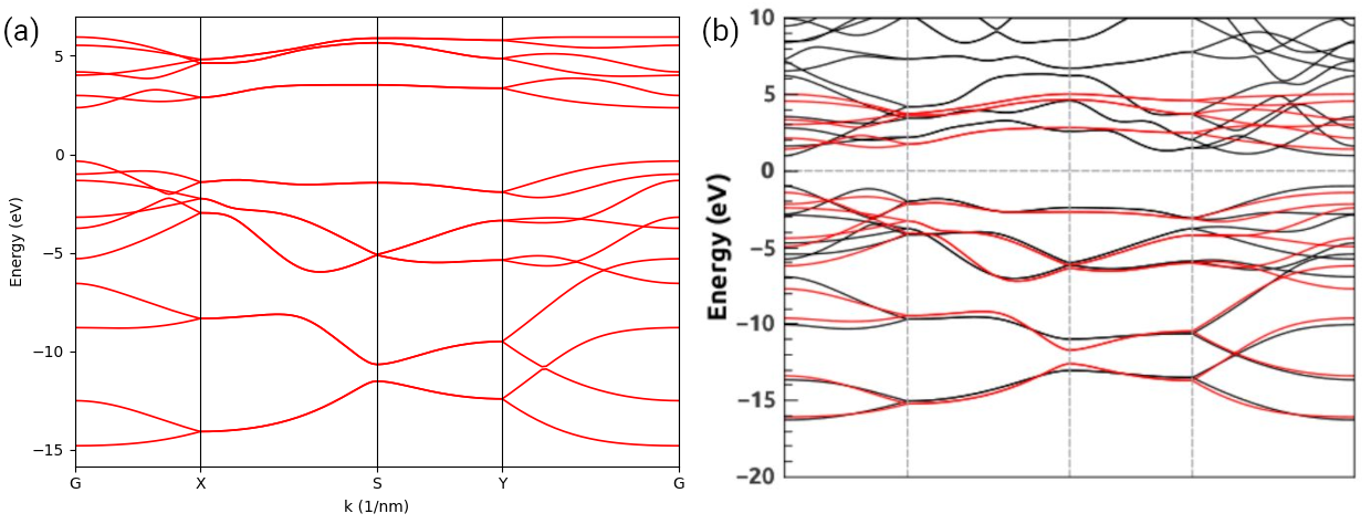
Band structure of monolayer graphene: (a) orthogonal basis set; (b) non-orthogonal basis set.