Plot 3D wavefunction
In this tutorial, we show how to plot the three-dimensional wavefunction and save it to Gaussaian
cube format. Cube is a common file format for representing volumic data in real space, and can be
visualized by a lot of tools like XCrySDen,
VESTA and Avogadro.
The Visualizer class offers a plot_wfc3d() function to plot the wavefunction
in cube format. We demonstrate its usage by visualizing the bonding and anti-bonding states of
hydrogen molecule, then the influence of k-point on the Bloch states of a hydrogen atom chain.
Finally, we turn to the more realistic graphene model and visualize its wavefunctions of different
Hamiltonian convention. To begin with, we import the necessary packages
import numpy as np

import tbplas as tb
H2 molecule
The bonding and anti-bonding states of a hydrogen molecule can be visualized as
 1"""Plot the bonding and anti-boding states of H2 molecule."""
 2# 1nm * 1nm * 1nm cubic cell
 3lattice = np.eye(3, dtype=np.float64)
 4h_bond = 0.074  # H-H bond length in nm
 5prim_cell = tb.PrimitiveCell(lattice, unit=tb.NM)
 6prim_cell.add_orbital((0.5-0.5*h_bond, 0.5, 0.5))
 7prim_cell.add_orbital((0.5+0.5*h_bond, 0.5, 0.5))
 8prim_cell.add_hopping((0, 0, 0), 0, 1, -1.0)
 9qn = np.array([(1, 1, 0, 0) for _ in range(prim_cell.num_orb)])
10
11# Calculate wave function
12k_points = np.array([[0.0, 0.0, 0.0]])
13solver = tb.DiagSolver(prim_cell)
14solver.config.prefix = "h2_molecule"
15solver.config.k_points = k_points
16bands, states = solver.calc_states()
17
18# Define plotting range
19# Cube volume: [0.25, 0.75] * [0.25, 0.75] * [0.25, 0.75] in nm
20cube_origin = np.array([0.25, 0.25, 0.25])
21cube_size = np.array([0.5, 0.5, 0.5])
22rn_max = np.array([0, 0, 0])
23
24# Plot wave function
25vis = tb.Visualizer()
26vis.plot_wfc3d(prim_cell, wfc=states[0, 0], quantum_numbers=qn,
27               convention=1, k_point=k_points[0], rn_max=rn_max,
28               cube_name="h2.bond.cube", cube_origin=cube_origin,
29               cube_size=cube_size, kind="abs2")
30vis.plot_wfc3d(prim_cell, wfc=states[0, 1], quantum_numbers=qn,
31               convention=1, k_point=k_points[0], rn_max=rn_max,
32               cube_name="h2.anti-bond.cube", cube_origin=cube_origin,
33               cube_size=cube_size, kind="abs2")
We define a \(1nm \times 1nm \times 1nm\) cubic cell to hold the molecule in line 3-4. In line 5-7 we add the two hydrogen atoms near the center of the cell. Then in line 8 we add the hopping term, which should be negative since it originates from the attractive Coulomb interaction between the electron and the nucleus. In line 9 we define the quantum number of the two \(1s\) states, where the first 1 indicate the nuclear charge \(Z\). The following 1 and 0 stand for the principle and angular quantum numbers \(n\) and \(l\). The last number 0 is the modified magnetic number \(\overline{m}\) indicating the kind of real spherical harmonics. The possible combinations of \(l\) and \(\overline{m}\) are
(0, 0): \(s\)
(1, -1): \(p_y\)
(1, 0): \(p_z\)
(1, 1): \(p_x\)
(2, -2): \(d_{xy}\)
(2, -1): \(d_{yz}\)
(2, 0): \(d_{z^2}\)
(2, 1): \(d_{xz}\)
(2, 2): \(d_{x^2-y^2}\)
(3, -3): \(f_{y(3x^2-y^2)}\)
(3, -2): \(f_{xyz}\)
(3, -1): \(f_{yz^2}\)
(3, 0): \(f_{z^3}\)
(3, 1): \(f_{xz^2}\)
(3, 2): \(f_{z(x^2-y^2)}\)
(3, 3): \(f_{x(x^2-3y^2)}\)
Then in 12-14 we calculate the wave functions for the \(\Gamma\) point since the hydrogen molecule is non-periodic. In line 18-19 we define the cube volume, which is located at \((0.25, 0.25, 0.25)\) and spans \(0.5 \times 0.5 \times 0.5\) (all units in nm). In line 20 we define the range of \(R\) in the evaluation of Bloch basis
in convention 1 and
in convention 2. Since out model is non-periodic, we restrict \(R\) to the \((0, 0, 0)\)
cell. In line 23-28 we plot the wavefunctions to cube files. The convention argument controls
the convention of Bloch basis, which should be consistent with the argument when calling
calc_states(). The kind argument defines which part of the wavefunction to plot,
which should be either “real”, “imag” or “abs2”. In our case we plot the squared norm of the
wavefunction. The output is shown in the figure below, where the bonding and anti-boding states
show significant charge accumulation and deleption in the internuclear area, respectively.
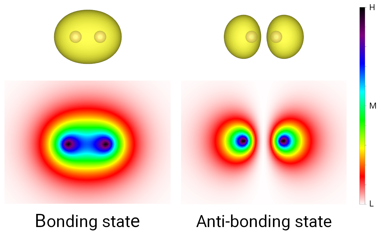
Bonding and anti-boding states of hydrogen molecule.
Hydrogen chain
The Bloch states in one-dimensional hydrogen chain can be visualized as
 1"""Plot the wave function of a hydrogen chain."""
 2# 0.074nm * 0.074nm * 0.074nm cubic cell
 3lattice = 0.074 * np.eye(3, dtype=np.float64)
 4prim_cell = tb.PrimitiveCell(lattice, unit=tb.NM)
 5prim_cell.add_orbital((0.0, 0.0, 0.0))
 6prim_cell.add_hopping((1, 0, 0), 0, 0, -1.0)
 7qn = np.array([(1, 1, 0, 0) for _ in range(prim_cell.num_orb)])
 8
 9# Calculate wave function
10k_points = np.array([[0.0, 0.0, 0.0]])
11solver = tb.DiagSolver(prim_cell)
12solver.config.prefix = "h2_chain"
13solver.config.k_points = k_points
14bands, states = solver.calc_states()
15
16# Define plotting range
17# Cube volume: [-0.75, 0.75] * [-0.25, 0.25] * [-0.25, 0.25] in nm
18cube_origin = np.array([-0.75, -0.25, -0.25])
19cube_size = np.array([1.5, 0.5, 0.5])
20rn_max = np.array([15, 0, 0])
21
22# Plot wave function
23vis = tb.Visualizer()
24vis.plot_wfc3d(prim_cell, wfc=states[0, 0], quantum_numbers=qn,
25               convention=1, k_point=k_points[0], rn_max=rn_max,
26               cube_name="h2_chain.cube", cube_origin=cube_origin,
27               cube_size=cube_size, kind="real")
Much of the code is similar to that of hydrogen molecule. We build a cubic cell with length of
0.074nm (bond length of hydrogen molecule), and add one atom at \((0, 0, 0)\). There is one
hopping term from the \((0, 0, 0)\) cell to the neighbouring \((1, 0, 0)\) cell. Since our
model is periodic this time, we set rn_max to (15, 0, 0) in line 18, which covers
neighbouring cells from \((-15, 0, 0)\) to \((15, 0, 0)\). The wavefunctions for different
k-points are shown as below. Since the k-point controls the wave vector in real space, we can see
a larger k leads to smaller wave lengths
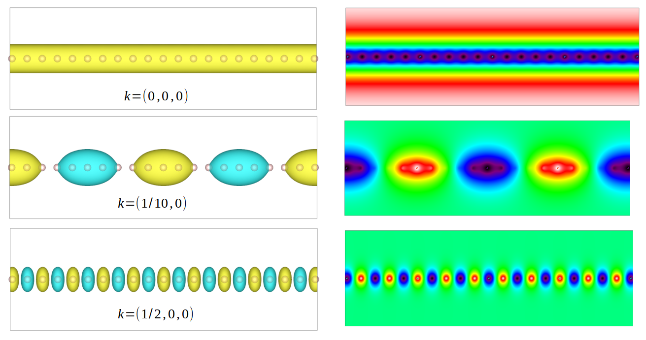
Wavefunctions of hydrogen chain for different k-points.
Graphene
Finally, we visualize the wavefunctions of monolayer graphene to see how the atomic positions and convention of Hamiltonian affect the spatial distribution of wavefunction.
 1"""Plot the wave function of monolayer graphene."""
 2vectors = tb.gen_lattice_vectors(a=0.246, b=0.246, gamma=60)
 3prim_cell = tb.PrimitiveCell(vectors, unit=tb.NM)
 4prim_cell.add_orbital((0.0, 0.0), label="C_pz")
 5prim_cell.add_orbital((1/3., 1/3.), label="C_pz")
 6prim_cell.add_hopping((0, 0), 0, 1, -2.7)
 7prim_cell.add_hopping((1, 0), 1, 0, -2.7)
 8prim_cell.add_hopping((0, 1), 1, 0, -2.7)
 9qn = np.array([(6, 2, 1, 0) for _ in range(prim_cell.num_orb)])
10
11# Calculate wave function
12k_points = np.array([[0.0, 0.0, 0.0]])
13solver = tb.DiagSolver(prim_cell)
14solver.config.prefix = "graphene"
15solver.config.k_points = k_points
16bands, states = solver.calc_states()
17
18# Define plotting range
19# Cube volume: [-0.75, 0.75] * [-0.75, 0.75] * [-0.25, 0.25] in nm
20cube_origin = np.array([-0.75, -0.75, -0.25])
21cube_size = np.array([1.5, 1.5, 0.5])
22rn_max = np.array([3, 3, 0])
23
24# Plot wave function
25vis = tb.Visualizer()
26vis.plot_wfc3d(prim_cell, wfc=states[0, 0], quantum_numbers=qn,
27               convention=1, k_point=k_points[0], rn_max=rn_max,
28               cube_name="graphene.cube", cube_origin=cube_origin,
29               cube_size=cube_size, kind="real")
We consider two different set of atomic positions, \((0, 0, 0)\) and \((\frac{1}{3}, \frac{1}{3}, 0)\), or \((\frac{1}{3}, \frac{1}{3}, 0)\) and \((\frac{2}{3}, \frac{2}{3}, 0)\). The k-points are \(\Gamma (0, 0, 0)\), \(K (\frac{1}{3}, \frac{2}{3}, 0)\) and \(M (\frac{1}{2}, 0, 0)\). The output are shown below. We can see the wavefunction at \(\Gamma\) point is irrelavant on atomic positions and Hamiltonian convention, since the phase vector is always 1. For other k-points, the wavefunction does not change on atomic positions for convention 2, since the phase factor involves only the cell index \(R\). For convention 1, either changing the atomic positions or the convention will change the wave function.
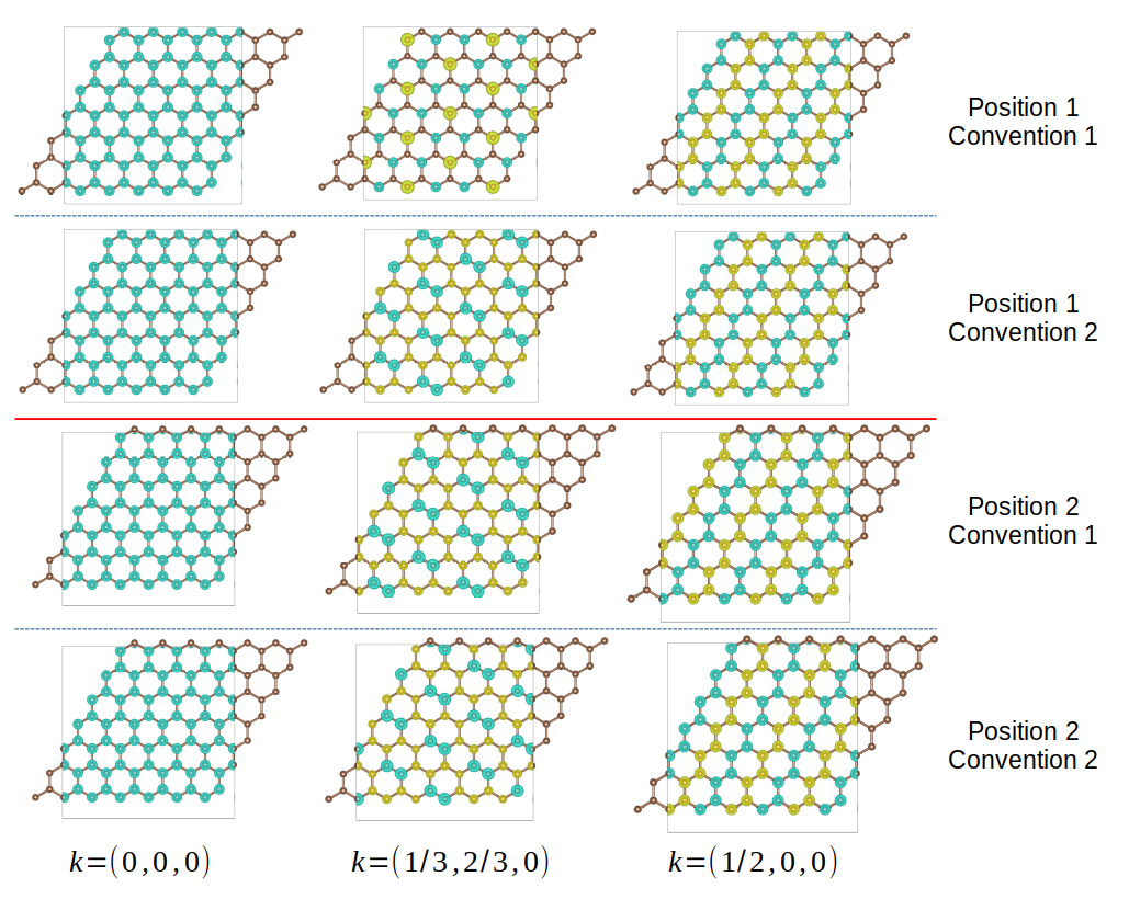
Wavefunctions of hydrogen chain for different k-points.