Quasi-eigenstates

The quasi-eigenstates are defined as

\[\begin{split}|\Psi(E) \rangle &=\frac{1}{2\pi} \int_{-\infty}^{\infty} \mathrm{e}^{\mathrm{i}Et} |\psi(t) \rangle \mathrm{d}t \nonumber \\ &=\frac{1}{2\pi}\sum_i a_i \int_{-\infty}^{\infty} \mathrm{e}^{\mathrm{i}(E-E_i)t} |\phi_i \rangle \mathrm{d}t \nonumber \\ &=\sum_i a_i \delta(E-E_i)|\phi_i \rangle\end{split}\]

If the energy \(E\) equals to an eigenvalue \(E_i\), then the quasi-eigenstate is the exact eigenstate corresponding to \(E_i\), or a superposition of degenerate eigenstates if \(E_i\) is degenerate. In this tutorial, we will show how to calculate the quasi-eigenstates and compare them with the exact eigenstates. The script can be found at examples/advanced/quasi_eigen.py. We begin with importing the necessary packages:

import numpy as np

import tbplas as tb

And define the following functions to generate primitive cell and sample with a single vacancy:

def make_prim_cell() -> tb.PrimitiveCell:
    """
    Make graphene primitive cell with a single vacancy.

    :return: primitive cell with vacancy
    """
    prim_cell = tb.make_graphene_diamond()

    # Get the index of vacancy
    dim = (17, 17, 1)
    orb_map = tb.RegularOrbitalMap(dim, prim_cell.num_orb)
    vac_id = orb_map.pc2sc(8, 8, 0, 0)

    # Extend cell and remove orbital
    prim_cell = tb.extend_prim_cell(prim_cell, dim=dim)
    prim_cell.remove_orbitals([vac_id])
    return prim_cell


def make_sample() -> tb.Sample:
    """
    Make graphene sample with a single vacancy.

    :return: sample with vacancy
    """
    prim_cell = tb.make_graphene_diamond()

    # Get the index of vacancy
    dim = (17, 17, 1)
    orb_map = tb.RegularOrbitalMap(dim, prim_cell.num_orb)
    vac_id = orb_map.pc2sc(8, 8, 0, 0)

    # Create supercell and sample
    super_cell = tb.SuperCell(prim_cell, dim=dim, pbc=(True, True, False),
                              vacancies=[vac_id])
    sample = tb.Sample(super_cell)
    return sample

We are going to create a \(17\times17\times1\) graphene sample with a vacancy in the center. We utilize the RegularOrbitalMap class to get the index of the 0th orbital in the \((8, 8, 0)\) cell. For the PrimitiveCell class, vacancies are added by calling the remove_orbitals method, while for the SuperCell class they are added via the vacancies argument.

Exact eigenstates

We define the following function to calculate the exact eigenstates:

def wfc_diag(prim_cell: tb.PrimitiveCell) -> None:
    """
    Calculate wave function using exact diagonalization.

    :param prim_cell: primitive cell
    :return: None
    """
    solver = tb.DiagSolver(prim_cell)
    solver.config.prefix = "diag"
    solver.config.k_points = np.array([[0.0, 0.0, 0.0]])
    bands, states = solver.calc_states()
    i_b = prim_cell.num_orb // 2
    wfc = np.abs(states[0, i_b])**2
    wfc /= wfc.max()
    vis = tb.Visualizer()
    vis.plot_wfc(prim_cell, wfc, scatter=True, site_size=wfc * 100, site_color="r",
                 with_model=True, model_style={"alpha": 0.25, "color": "gray"},
                 fig_name="diag.png", fig_size=(6, 4.5), fig_dpi=100)

In line 8 we create the solver from DiagSolver class. Then we define the prefix of data files and the k-points on which the eigenstates will be calculated in line 9-10, where we consider the \(\Gamma\) point. In line 11 we call the calc_states method to get the eigenvalues and eigenstates, as returned in bands and states. After that, we extract the eigenstate at the Fermi level and normalize it in line 12-14. To visualize the eigenstate, we create a visualizer from the Visualizer class and call its plot_wfc method. Note that we must use scatter plot by setting the scatter argument to true. The eigenstate should be passed as the site_size argument, i.e., sizes of scatters will indicate the projection of eigenstate on the sites. We also need to show the model alongside the eigenstate through the with_model argument and define its plotting style with the model_style argument.

Quasi-eigenstates

The quasi-eigenstate is evaluated and plotted in a similar approach:

def wfc_tbpm(sample: tb.Sample) -> None:
    """
    Calculate wave function using TBPM.

    :param sample: graphene sample
    :return: None
    """
    solver = tb.TBPMSolver(sample)
    solver.config.prefix = "tbpm"
    solver.config.rescale = 9.0
    solver.config.num_random_samples = 1
    solver.config.num_time_steps = 1024
    solver.config.qe_energies = np.array([0.0])
    qs = solver.calc_quasi_eigenstates()
    wfc = qs[0]  # qs is already the squared norm
    wfc /= wfc.max()
    vis = tb.Visualizer()
    vis.plot_wfc(sample, wfc, scatter=True, site_size=wfc*100, site_color="b",
                 with_model=True, model_style={"alpha": 0.25, "color": "gray"},
                 fig_name="tbpm.png", fig_size=(6, 4.5), fig_dpi=100)

Evaluating quasi-eigenstates is a kind of TBPM calculation, so it follows the common procedure of TBPM. We firstly create the solver from TBPMSolver class in line 8, then set the calculation parameters in line 9-13. Especially, the qe_energies argument defines the energies for which the quasi-eigenstates will be evaluated. Then we call the calc_quasi_eigenstates method of TBPMSolver to get the eigenstates, normalize it, and visualize it in line 14-20.

Finally, we define the driving function:

def main():
    wfc_diag(make_prim_cell())
    wfc_tbpm(make_sample())


if __name__ == "__main__":
    main()

The output is shown in Fig. 1. It is clear that the eigenstate and quasi-eigenstate are localized around the vacancy with a 3-fold rotational symmetry.

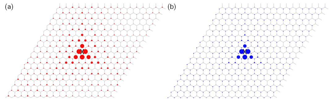
Spatial distribution of (a) exact eigenstate and (b) quasi-eigenstate of graphene sample with a vacancy in the center. The X marks indicate the position of the vacancy.