Bands and DOS

In this tutorial, we show how to calculate the band structure and density of states of a sample via exact diagonalization. The Sample class shares the same APIs for obtaining these properties as PrimitiveCell class, so the procedure in Band structure and DOS is directly applicable. The scripts can be found at examples/sample/band_dos.

Band structure of graphene nano-ribbon

For convenience, we reuse the models in Set up the sample:

import numpy as np
import tbplas as tb

rect_cell = tb.make_graphene_rect()
sc_am = tb.SuperCell(rect_cell, dim=(3, 3, 1), pbc=(False, True, False))
gnr_am = tb.Sample(sc_am)
sc_zz = tb.SuperCell(rect_cell, dim=(3, 3, 1), pbc=(True, False, False))
gnr_zz = tb.Sample(sc_zz)

The band structure of armchair-edged nano-ribbon can be obtained as:

k_points = np.array([
    [0.0, -0.5, 0.0],
    [0.0, 0.0, 0.0],
    [0.0, 0.5, 0.0],
])
k_label = ["X", "G", "X"]
k_path, k_idx = tb.gen_kpath(k_points, [40, 40])
k_len, bands = gnr_am.calc_bands(k_path)
vis = tb.Visualizer()
vis.plot_bands(k_len, bands, k_idx, k_label)

For zigzag-edged nano-ribbon, k_points should be replaced with:

k_points = np.array([
    [-0.5, 0.0, 0.0],
    [0.0, 0.0, 0.0],
    [0.5, 0.0, 0.0],
])

The output is shown in the figure, consistent with Build complex primitive cells.

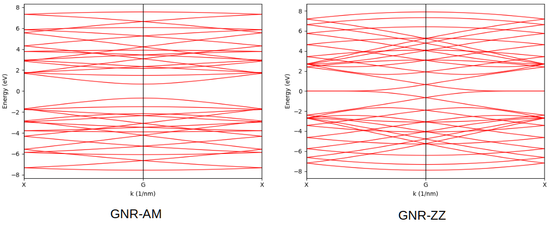
Band structures of armchair and zigag-edged graphene nano-ribbons.

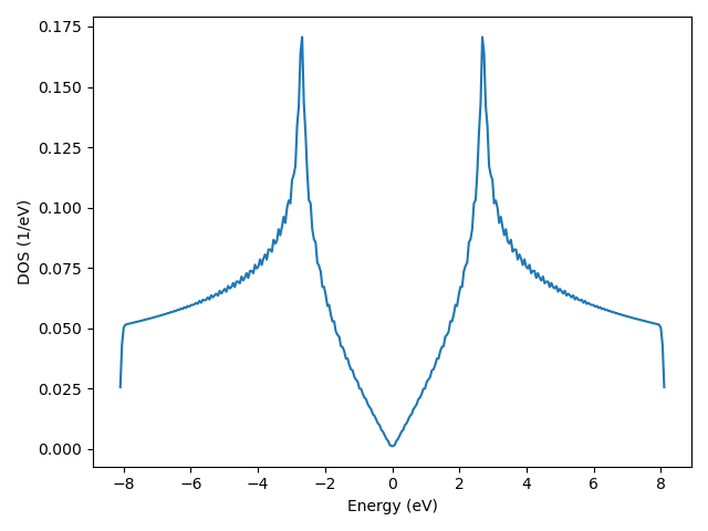
DOS of graphene

In Band structure and DOS we have calculated the DOS of a graphene primitive cell with a kgrid of 120*120*1. This is equivalent to evaluate the DOS of a graphene sample consisting of 20*20*1 cells with 6*6*1 kgrid:

import numpy as np
import tbplas as tb

prim_cell = tb.make_graphene_diamond()
sc = tb.SuperCell(prim_cell, dim=(20, 20, 1), pbc=(True, True, False))
sample = tb.Sample(sc)

k_mesh = tb.gen_kmesh((6, 6, 1))
energies, dos = sample.calc_dos(k_mesh)

vis = tb.Visualizer()
vis.plot_dos(energies, dos)