Spin texture
In this tutorial, we demonstrate the usage of SpinTexture class by calculating the spin
texture of graphene with Rashba and Kane-Mele spin-orbital coupling. The spin texture is defined
as the the expectation of Pauli operator \(\sigma_i\), which can be considered as a function of
band index \(n\) and \(\mathbf{k}\)-point
where \(i \in {x, y, z}\) are components of the Pauli operator. The spin texture can be evaluated
for given band index \(n\) or fixed energy, while in this tutorial we will focus on the former
case. The script is located at examples/prim_cell/spin_texture/spin_texture.py. As in other tutorials,
we begin with importing the tbplas package:
import tbplas as tb
Evaluation of spin texture
We evaluation of spin texture in the following manner:
 1# Import the model and define some parameters
 2cell = tb.make_graphene_soc(is_qsh=True)
 3ib = 2
 4spin_major = False
 5
 6# Evaluate expectation of sigma_z
 7k_grid = 2 * tb.gen_kmesh((240, 240, 1)) - 1
 8spin_texture = tb.SpinTexture(cell, k_grid, spin_major)
 9k_cart = spin_texture.k_cart
10sz = spin_texture.eval("z")
11vis = tb.Visualizer()
12vis.plot_scalar(x=k_cart[:, 0], y=k_cart[:, 1], z=sz[:, ib],
13                num_grid=(480, 480), cmap="jet")
14
15# Evaluate expectation of sigma_x and sigma_y
16k_grid = 2 * tb.gen_kmesh((48, 48, 1)) - 1
17spin_texture.k_grid = k_grid
18k_cart = spin_texture.k_cart
19sx = spin_texture.eval("x")
20sy = spin_texture.eval("y")
21vis.plot_vector(x=k_cart[:, 0], y=k_cart[:, 1], u=sx[:, ib], v=sy[:, ib],
22                cmap="jet")
In line 2 we import the graphene model with Rashba and Kane-Mele SOC with the make_graphene_soc()
function. In line 3-4 we define the band index and whether the orbitals are sorted in spin-major order,
which will be discussed in more details in the next section. To plot the expectation of \(\sigma_i\)
as function of \(\mathbf k\)-point, we need to generate a uniform meshgrid in the Brillouin zone. As
the gen_kmesh() function generates k-grid on \([0, 1]\), so we need to multiply the result by
a factor of 2, then extract 1 from it such that the k-grid will be on \([-1, 1]\) which is enough to
cover the first Brillouin zone. Then we create a SpinTexture object in line 8. In line 9-10 we
get the Cartesian coordinates of k-grid and the expectation of \(\sigma_z\), and visualize it in line
11-13 as colormap using the plot_scalar method. The argument ib specifies the band index \(n\)
to plot. The result is shown in Fig. 1(a).
The evaluation of \(\sigma_x\) and \(\sigma_y\) is similar. In line 16-17 we assign a more sparse
k-grid to the SpinTexture object since we are going to plot the expectation as vector field. In
18-20 we get the Cartesian coordinates of k-grid and the expectation of \(\sigma_x\) and \(\sigma_y\),
and plot them as vector field in line 21-22. The output is shown in Fig. 1(b).
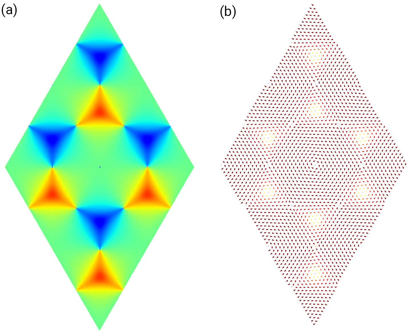
Plot of expectation of (a) \(\sigma_z\) and (b) \(\sigma_x\) and \(\sigma_y\).
Orbital order
The order of spin-polarized orbitals determines how the spin-up and spin-down components are extracted from the
eigenstates. There are two popular orders: spin-major and orbital-major. For example, there are two \(p_z\)
orbitals in the two-band model of monolayer graphene in the spin-unpolarized case, which can be denoted as
\(\{\phi_1, \phi_2\}\). When spin has been taken into consideration, the orbitals become
\(\{\phi_1^{\uparrow}, \phi_2^{\uparrow}, \phi_1^{\downarrow}, \phi_2^{\downarrow}\}\). In spin-major order
they are sorted as \([\phi_1^{\uparrow}, \phi_2^{\uparrow}, \phi_1^{\downarrow}, \phi_2^{\downarrow}]\),
while in orbital-major order they are sorted as
\([\phi_1^{\uparrow}, \phi_1^{\downarrow}, \phi_2^{\uparrow}, \phi_2^{\downarrow}]\). The split_spin
method of SpinTexture class extracts the spin-up and spin-down components as following:
 1def split_spin(self, state: np.ndarray) -> Tuple[np.ndarray, np.ndarray]:
 2    """
 3    Split spin-up and spin-down components for wave function at given
 4    k-point and band.
 5
 6    Two kinds of orbital orders are implemented:
 7    spin major: psi_{0+}, psi_{1+}, psi_{0-}, psi_{1-}
 8    orbital major: psi_{0+}, psi_{0-}, psi_{1+}, psi_{1-}
 9
10    If the orbitals are sorted in neither spin nor orbital major,
11    derive a new class from SpinTexture and overwrite this method.
12
13    :param state: (num_orb,) complex128 array
14        wave function at given k-point and band
15    :return: (u, d)
16        u: (num_orb//2,) complex128 array
17        d: (num_orb//2,) complex128 array
18        spin-up and spin-down components of the wave function
19    """
20    num_orb = self.num_orb // 2
21    if self._spin_major:
22        u, d = state[:num_orb], state[num_orb:]
23    else:
24        u, d = state[0::2], state[1::2]
25    return u, d
If the spin-polarized orbitals follow other user-defined orders, then the users should derive their
own class from SpinTexture and overload the split_spin method.