Setting up the primitive cell
In this tutorial, we show how to set up the primitive cell from the PrimitiveCell class taking
monolayer graphene as the example. We will discuss the geometric properties of graphene first, then
set up the model step-by-step. The script in this tutorial can be found at
examples/prim_cell/model/graphene_diamond.py.
Geometric properties
Monolayer graphene has a hexagonal lattice, with lattice parameters \(a=b=2.46 \overset{\circ}{\mathrm {A}}\) and \(\alpha=\beta=90^\circ\). The angle between lattice vectors \(a_1\) and \(a_2\), namely \(\gamma\), can be either \(60^\circ\) or \(120^\circ\), depending on the choice of lattice vectors, as shown in the figure:
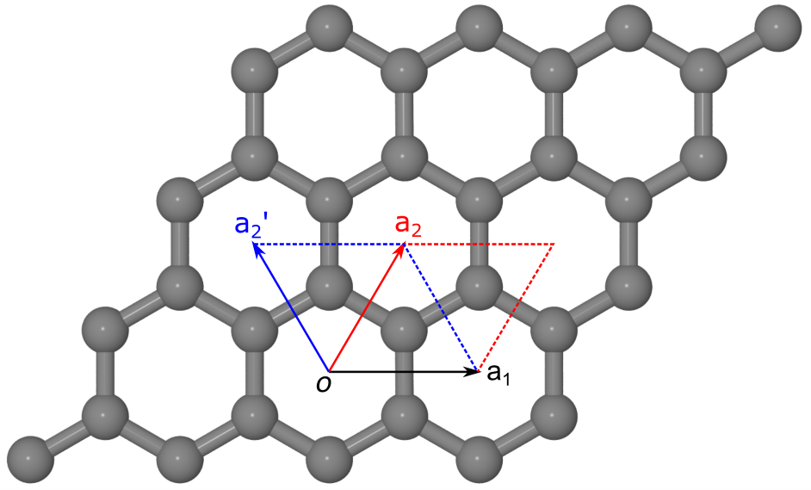
Crystalline structure of monolayer graphene. Grey spheres indicate the carbon atoms. \((a_1, a_2)\) and \((a_1, a_2\prime)\) are two equivalent sets of lattice vectors, with the angle \(\gamma\) being either \(60^\circ\) or \(120^\circ\). The corresponding primitive cells are indicated with red and blue diamonds, respectively.
Each primitive cell of monolayer graphene has two carbon atoms located at
\(\tau_1 = \frac{1}{3}a_1 + \frac{1}{3}a_2\)
\(\tau_2 = \frac{2}{3}a_1 + \frac{2}{3}a_2\)
if \(\gamma=60^\circ\) and
\(\tau_1 = \frac{2}{3}a_1 + \frac{1}{3}a_2\)
\(\tau_2 = \frac{1}{3}a_1 + \frac{2}{3}a_2\)
if \(\gamma=120^\circ\). We call the coordinates of \((\frac{1}{3}, \frac{1}{3}) (\frac{2}{3}, \frac{2}{3})\)
and \((\frac{2}{3}, \frac{1}{3}) (\frac{1}{3}, \frac{2}{3})\) as fractional coordinates. If you are familiar with
density functional theory programs, e.g. VASP and Quantum ESPRESSO, you will immediately see that they are the direct
or crystal coordinates. The advantage of fractional coordinates is that they are compact and independent of the orientation
of lattice vectors. The PrimitiveCell class of TBPLaS uses fractional coordinates internally, yet there are
utilities to convert them from/to Cartesian coordinates.
Create empty cell
First of all, we need to import all necessary packages:
import math
import numpy as np
import tbplas as tb
To create an empty primitive cell, we need to define of lattice vectors. We choose \(\gamma=60^\circ\).
Since all cells are implemented as 3-dimensional within TBPLaS, we need to specify an arbitrary lattice constant c,
which is taken to be \(10\overset{\circ}{\mathrm {A}}\). The empty cell can be generated by the following function:
def make_empty_cell(algo: int = 0) -> tb.PrimitiveCell:
    """
    Generate lattice vectors of monolayer graphene.
    :param algo: algorithm to generate lattice vectors
    :return: empty primitive cell
    """
    a = 2.46  # cell length a in Angstrom
    b = a  # cell length b in Angstrom
    c = 10.0  # cell length c in Angstrom
    gamma = 60.0  # angle between a1 and a2 in Degrees
    a_half = a * 0.5
    sqrt3 = math.sqrt(3)
    if algo == 0:
        vectors = tb.gen_lattice_vectors(a=a, b=b, c=c, gamma=gamma)
    elif algo == 1:
        vectors = np.array([
            [a, 0, 0,],
            [a_half, sqrt3*a_half, 0],
            [0, 0, c]])
    else:
        vectors = np.array([
            [sqrt3*a_half, -a_half, 0],
            [sqrt3*a_half, a_half, 0],
            [0, 0, c]])
    cell = tb.PrimitiveCell(vectors, unit=tb.ANG)
    return cell
We can generate the lattice vectors from lattice functions by calling gen_lattice_vectors() (algo=0),
or input the Cartesian coordinates manually (algo=1 and algo=2). Note that the orientation of the lattice
vectors is arbitrary, and we have \(a_1\) parallel to \(x\)-axis (algo=1). We can also make
\(a_1\) and \(a_2\) to be symmetric about \(x\)-axis (algo=2). When the lattice vectors are ready,
we create an empty primitive cell from the PrimitiveCell class. The unit argument specifying the unit of Cartesian coordinates of lattice vectors.
Add orbitals
Since we choose \(\gamma=60^\circ\), the two carbon atoms are then located at \((\frac{1}{3}, \frac{1}{3})\) and \((\frac{2}{3}, \frac{2}{3})\). In the simplest 2-band model of graphene, each carbon atom carries one \(p_z\) orbital. We define the following function to add the orbitals:
def add_orbitals(cell: tb.PrimitiveCell, algo: int = 0) -> None:
    """
    Add orbitals to the model.
    :param algo: algorithm to add orbitals
    :return: None. The incoming cell is modified.
    """
    if algo == 0:
        cell.add_orbital((1./3, 1./3),  energy=0.0, label="pz")
        cell.add_orbital((2./3, 2./3),  energy=0.0, label="pz")
    elif algo == 1:
        cell.add_orbital((1./3, 1./3, 0.5), energy=0.0, label="pz")
        cell.add_orbital((2./3, 2./3, 0.5), energy=0.0, label="pz")
    else:
        # NOTE: Tt is assumed that a_1 should be parallel to x-axis
        cell.add_orbital_cart((1.23, 0.71014083), unit=tb.ANG, energy=0.0, label="pz")
        cell.add_orbital_cart((2.46, 1.42028166), unit=tb.ANG, energy=0.0, label="pz")
We can add the orbitals using fractional coordinates (algo=0 and algo=1). The fractional coordinate along c-axis
is assumed to 0 if not specified (algo=0). We can also make the orbitals to be located at
\(z=0.5\times10\overset{\circ}{\mathrm {A}} = 5\overset{\circ}{\mathrm {A}}\) (algo=1).
The parameter energy gives the on-site energy of the orbital, which is assumed to be 0 eV if not specified. In absence
of strain or external fields, the two orbitals have the same on-site energy. The parameter label is a tag to label
the orbital.
In addition to fractional coordinates, the orbitals can also be added using Cartesian coordinates (algo=2).
Here we use the parameter unit to specify the unit of the Cartesian coordinates. Note that PrimitiveCell
class always uses fractional coordinates internally.
Add hopping terms
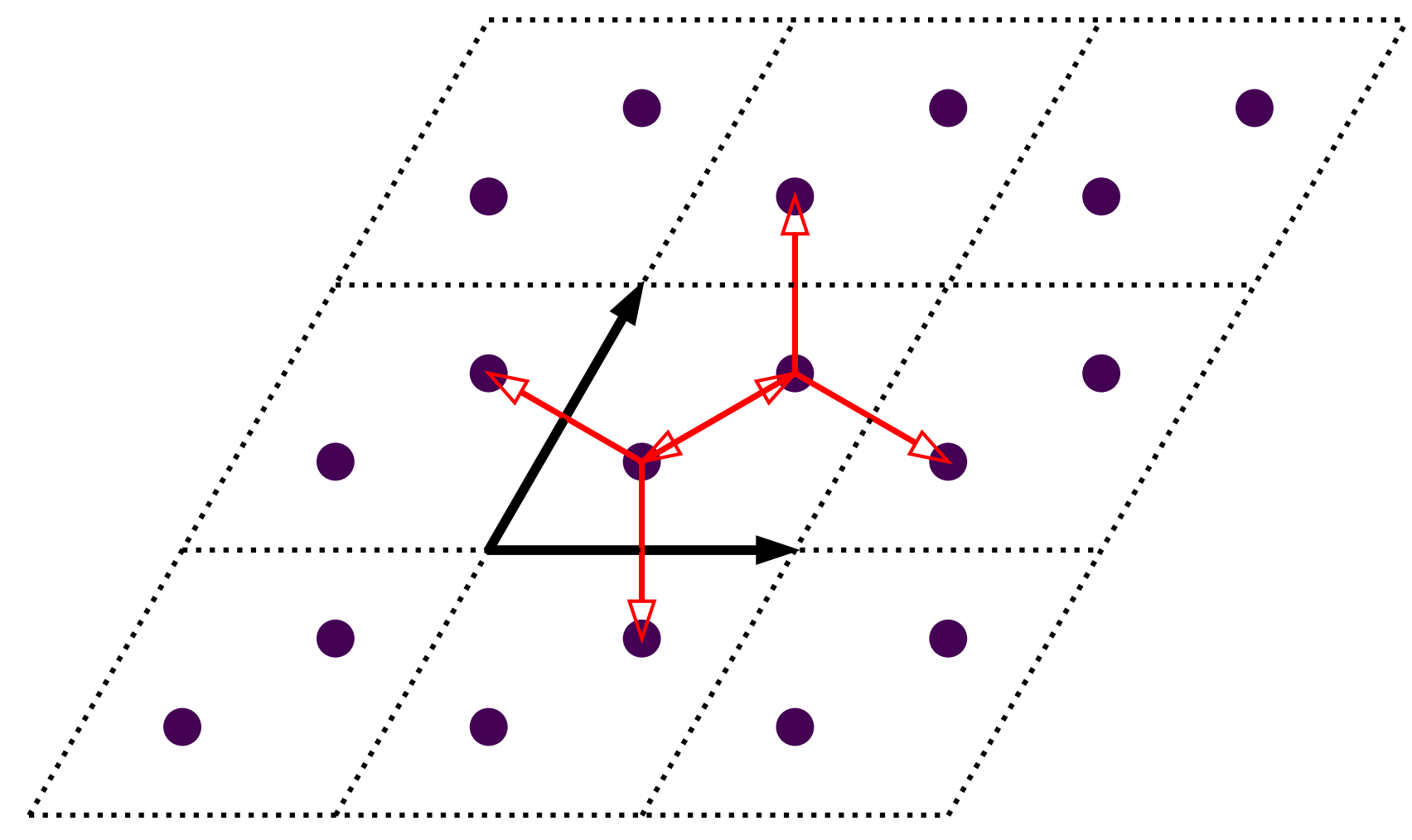
With the orbitals ready, we can add the hopping terms. The hopping terms for primitive cell with \(\gamma=60^\circ\) is shown in the figure below:

Schematic plot of hopping terms of graphene. Primitive cells are indicated with dashed diamonds and numbered in blue text. Thick black arrows indicate the lattice vectors. Orbitals and hopping terms are shown as filled circles and red arrows, respectively.
From the figure we can see there are 6 hopping terms between \((0, 0)\) and neighbouring cells in the nearest approximation:
\((0, 0) \rightarrow (0, 0), i=0, j=1\)
\((0, 0) \rightarrow (0, 0), i=1, j=0\)
\((0, 0) \rightarrow (1, 0), i=1, j=0\)
\((0, 0) \rightarrow (-1, 0), i=0, j=1\)
\((0, 0) \rightarrow (0, 1), i=1, j=0\)
\((0, 0) \rightarrow (0, -1), i=0, j=1\)
Using the conjugate relation \(\langle i, 0 | \hat{H} | j, R\rangle = \langle j, 0 | \hat{H} | i, -R\rangle^*\) they can be reduced to:
\((0, 0) \rightarrow (0, 0), i=0, j=1\)
\((0, 0) \rightarrow (1, 0), i=1, j=0\)
\((0, 0) \rightarrow (0, 1), i=1, j=0\)
TBPLaS utilities the conjugate relation, so we need only to provide the reduced hopping terms.
The hopping terms can be added with the following function:
def add_hopping_terms(cell: tb.PrimitiveCell, algo: int = 0) -> None:
    """
    Add hopping terms the model.
    :param algo: algorithm to add hopping terms
    :return: None. The incoming cell is modified.
    """
    if algo == 0:
        cell.add_hopping(rn=(0, 0), orb_i=0, orb_j=1, energy=-2.7)
        cell.add_hopping(rn=(1, 0), orb_i=1, orb_j=0, energy=-2.7)
        cell.add_hopping(rn=(0, 1), orb_i=1, orb_j=0, energy=-2.7)
    else:
        cell.add_hopping(rn=(0, 0, 0), orb_i=0, orb_j=1, energy=-2.7)
        cell.add_hopping(rn=(1, 0, 0), orb_i=1, orb_j=0, energy=-2.7)
        cell.add_hopping(rn=(0, 1, 0), orb_i=1, orb_j=0, energy=-2.7)
The parameter rn specifies the index of neighboring cell, while orb_i and orb_j give the indices of orbitals
of the hopping term. energy is the hopping integral, which should be a complex number in general cases. The 3rd
component of rn is assumed to be 0 if not provided (algo=0). We can also specify it explicitly (algo=1).
Since monolayer graphene is two-dimensional, the 3rd component of rn is of course 0. In general cases it should
be non-zero.
Dump the model
Now we call all the functions to build the model:
cell = make_empty_cell(algo=0)
add_orbitals(cell, algo=0)
add_hopping_terms(cell, algo=0)
We can have a look at it by calling the plot method:
and print the orbitals and hopping terms by calling the print method. The output should look like:
Lattice origin (nm):
    0.00000   0.00000   0.00000
Lattice vectors (nm):
    0.24600   0.00000   0.00000
    0.12300   0.21304   0.00000
    0.00000   0.00000   1.00000
Orbitals:
    0.33333   0.33333   0.00000   0.00000
    0.66667   0.66667   0.00000   0.00000
Hopping terms:
    (0, 0, 0) (0, 1) -2.7
    (1, 0, 0) (1, 0) -2.7
    (0, 1, 0) (1, 0) -2.7
We can also get analytical Hamiltonian of the model by calling the print_hk method:
ham[0, 0] = (0.0)
ham[1, 1] = (0.0)
ham[0, 1] = ((-2.7+0j) * exp_i(0.3333333333333333 * ka + 0.3333333333333333 * kb)
+ (-2.7-0j) * exp_i(-0.6666666666666666 * ka + 0.3333333333333333 * kb)
+ (-2.7-0j) * exp_i(0.3333333333333333 * ka - 0.6666666666666666 * kb))
ham[1, 0] = ham[0, 1].conjugate()
with exp_i(x) := cos(2 * pi * x) + 1j * sin(2 * pi * x)
which accepts an convention argument defining the convention of Hamiltonian, as discussed in
Background. The Python and C++ code snippets to rebuilt the model can be obtained by the
print_py and print_cxx methods, respectively:
# Lattice vectors and origin.
lat_vec = np.array([
[  0.246 ,  0.0 ,  0.0 ,],
[  0.12300000000000003 ,  0.21304224933097193 ,  0.0 ,],
[  6.123233995736766e-17 ,  3.5352507957496895e-17 ,  1.0 ,],
])
origin = np.array([0.0, 0.0, 0.0])

# Create the primitive cell and set orbitals.
prim_cell = PrimitiveCell(lat_vec, origin, unit=1.0)
prim_cell.add_orbital((0.3333333333333333, 0.3333333333333333, 0.0), 0.0, 'pz')
prim_cell.add_orbital((0.6666666666666666, 0.6666666666666666, 0.0), 0.0, 'pz')

# Add hopping terms.
prim_cell.add_hopping((0, 0, 0), 0, 1, -2.7)
prim_cell.add_hopping((1, 0, 0), 1, 0, -2.7)
prim_cell.add_hopping((0, 1, 0), 1, 0, -2.7)

return prim_cell
// Lattice vectors and origin.
Eigen::Matrix3d lat_vec{
{  0.246 ,  0.0 ,  0.0 },
{  0.12300000000000003 ,  0.21304224933097193 ,  0.0 },
{  6.123233995736766e-17 ,  3.5352507957496895e-17 ,  1.0 }
};
Eigen::Vector3d origin(0.0, 0.0, 0.0);

// Create the primitive cell and set orbitals.
PrimitiveCell<complex_t> prim_cell(2, lat_vec, origin, 1.0);
prim_cell.set_orbital(0, 0.3333333333333333, 0.3333333333333333, 0.0, 0.0, 0);
prim_cell.set_orbital(1, 0.6666666666666666, 0.6666666666666666, 0.0, 0.0, 0);

// Add hopping terms.
prim_cell.add_hopping(0, 0, 0, 0, 1, { -2.7 ,  0.0 });
prim_cell.add_hopping(1, 0, 0, 1, 0, { -2.7 ,  0.0 });
prim_cell.add_hopping(0, 1, 0, 1, 0, { -2.7 ,  0.0 });

return prim_cell;