Band structure and DOS
In this tutorial, we show how to calculate the band structure and density of states (DOS) of a primitive cell
using monolayer graphene as the example. The script can be found at examples/prim_cell/band_dos/graphene.py.
First of all, we need to import all necessary packages:
import numpy as np
import matplotlib.pyplot as plt
import tbplas as tb
Of course, we can reuse the model built in Setting up the primitive cell. But this time we will import it from the materials repository for convenience:
cell = tb.make_graphene_diamond()
Band structure
The first Brillouin zone of a hexagonal lattice with \(\gamma=60^\circ\) is shown as below:
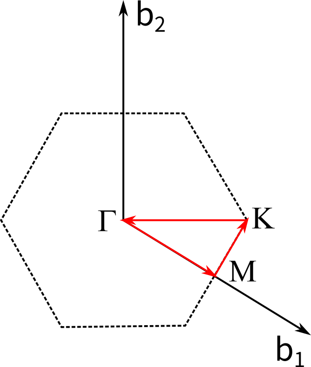
Schematic plot of the first Brillouin zone of a hexagonal lattice. \(b_1\) and \(b_2\) are basis vectors of reciprocal lattice. Dashed hexagon indicates the edges of first Brillouin zone. The path of \(\Gamma \rightarrow M \rightarrow K \rightarrow \Gamma\) is indicated with red arrows.
We generate a path of \(\Gamma \rightarrow M \rightarrow K \rightarrow \Gamma\), with 40 interpolated k-points along each segment, using the following commands:
k_points = np.array([
    [0.0, 0.0, 0.0],    # Gamma
    [1./2, 0.0, 0.0],   # M
    [2./3, 1./3, 0.0],  # K
    [0.0, 0.0, 0.0],    # Gamma
])
k_label = ["G", "M", "K", "G"]
k_path, k_idx = tb.gen_kpath(k_points, [40, 40, 40])
Here k_points is an array contaning the fractional coordinates of highly-symmetric k-points, which
are then passed to gen_kpath() for interpolation. k_path is an array containing interpolated
coordinates and k_idx contains the indices of highly-symmetric k-points in k_path. k_label
is a list of strings to label the k-points in the plot of band structure.
There are two approaches to evaluate the band structure:
use_diag_solver = True
if use_diag_solver:
    solver = tb.DiagSolver(cell)
    solver.config.k_points = k_path
    solver.config.prefix = "graphene"
    k_len, bands = solver.calc_bands()
else:
    k_len, bands = tb.calc_bands(cell, k_path, prefix="graphene")
The formal and recommended approach is to create a solver from the DiagSolver class and call the
calc_bands method (use_diag_solver=True). The other approach is to call the calc_bands()
function (use_diag_solver=True), which is a wrapper over DiagSolver. For both approaches,
we need to set the calculation parameters. In the first approach, this is done by modifying the attributes
of the config attribute of the solver, which is an instance of DiagConfig class. In the second
approach, this is done through keyword arguments of the function. We need to set the k-points and the prefix of data files.
After the band structure is obtained, it can be plotted by calling the plot_bands method of Visualizer class:
vis = tb.Visualizer()
vis.plot_bands(k_len, bands, k_idx, k_label)
or alternatively, using matplotlib directly:
num_bands = bands.shape[1]
for i in range(num_bands):
    plt.plot(k_len, bands[:, i], color="r", linewidth=1.0)
for idx in k_idx:
    plt.axvline(k_len[idx], color='k', linewidth=1.0)
plt.xlim((0, np.amax(k_len)))
plt.xticks(k_len[k_idx], k_label)
plt.xlabel("k (1/nm)")
plt.ylabel("Energy (eV)")
plt.tight_layout()
plt.show()
plt.close()
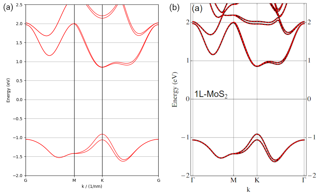
Band structure of monolayer graphene.
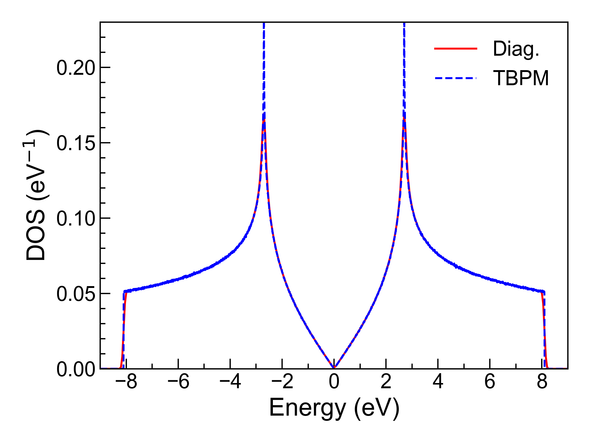
Density of states
To evaluate density of states (DOS) we need to generate a uniform k-mesh in the first Brillouin zone using the
gen_kmesh() function:
k_mesh = tb.gen_kmesh((120, 120, 1)) # 120*120*1 uniform meshgrid
Similar to band structure, there also two approaches to evaluate DOS, using either the calc_dos method
of DiagSolver class, or call the calc_dos() function directly:
if use_diag_solver:
    solver = tb.DiagSolver(cell)
    solver.config.k_points = k_mesh
    solver.config.prefix = "graphene"
    solver.config.e_min = -10
    solver.config.e_max = 10
    energies, dos = solver.calc_dos()
else:
    energies, dos = tb.calc_dos(cell, k_mesh, prefix="graphene", e_min=-10, e_max=10)
For both methods, we need specify the k-points, the prefix and the lower and upper bounds of the energy range.
Then we can visualize DOS with the plot_dos method of Visualizer class:
vis = tb.Visualizer()
vis.plot_dos(energies, dos)
Of course, we can also plot DOS using matplotlib directly:
plt.plot(energies, dos, color="r", linewidth=1.0)
plt.xlabel("Energy (eV)")
plt.ylabel("DOS (1/eV")
plt.tight_layout()
plt.show()
plt.close()