Properties from TBPM

In this tutorial, we demonstrate the usage of Tight-Binding Propagation Methods (TBPM) implemented in TBPLaS. TBPM can solve a lot of electronic and response properties of large tight-binding models in a much faster way than exact diagonalization. For the capabilities of TBPM, see Features. All TBPM calculations begin with setting up a sample from the Sample class, followed by specifying the configurations controlling the calculation using the Config class. From the sample and configurations a solver and an analyzer will be created from Solver and Analyzer classes, respectively. The solver is utilized to evaluate correlation functions, which are then analyzed by the analyzer to yield desired properties. Finally, the results are visualized by a visualizer of the Visualizer class or by matplotlib.

DOS of graphene

We begin with calculating the density of states of monolayer graphene. The script can be found at examples/sample/tbpm/graphene.py. Firstly, we create a graphene sample with 480*480*1 cells:

import matplotlib.pyplot as plt
import tbplas as tb

prim_cell = tb.make_graphene_diamond()
super_cell = tb.SuperCell(prim_cell, dim=(480, 480, 1), pbc=(True, True, False))
sample = tb.Sample(super_cell)
sample.rescale_ham(9.0)

The propagation of wave function is simulated with the algorithm of Chebyshev decomposition of Hamiltonian, which requires the eigenvalues of Hamiltonian to be on the range of \([-1, 1]\). So we need to rescale the Hamiltonian by calling the rescale_ham() method of Sample class. A scaling factor, e.g. 9.0 in the example, can be supplied to the function. If not given, the scaling factor will be estimated by inspecting the Hamiltonian automatically.

The parameters controlling TBPM calculations are stored in an instance of Config class:

config = tb.Config()
config.generic['nr_random_samples'] = 4
config.generic['nr_time_steps'] = 256

In the first line we create an instance of Config class. Then we specify that we are going to use 4 initial conditions. For each initial condition, the wave function will propagate 256 steps. From sample and config we can create the solver and analyzer, from Solver and Analyzer classes, respectively:

solver = tb.Solver(sample, config)
analyzer = tb.Analyzer(sample, config)

Then we can evaluate and analyze the correlation function:

corr_dos = solver.calc_corr_dos()
energies_dos, dos = analyzer.calc_dos(corr_dos)

And visualize the results:

plt.plot(energies_dos, dos)
plt.xlabel("Energy (eV)")
plt.ylabel("DOS")
plt.savefig("DOS.png")
plt.close()

The output is shown in panel (a) of the figure:

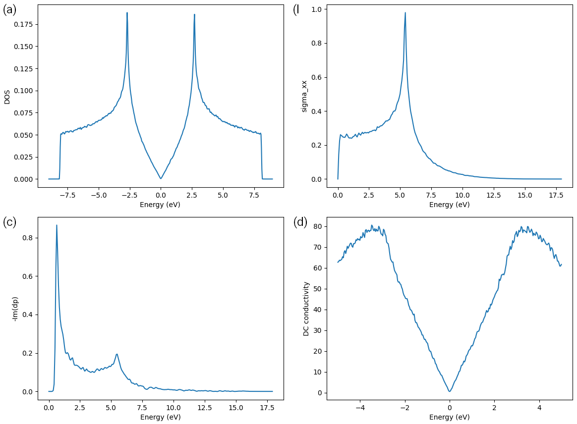
Density of states (a), optical (AC) conductivity (b), dynamic polarizability (c) and electronic (DC) conductivity (d) of graphene sample.

More properties from TBPM

We then demonstrate more capabilities of TBPM. Firstly, we add more settings to config:

config.generic['correct_spin'] = True
config.dyn_pol['q_points'] = [[1., 0., 0.]]
config.DC_conductivity['energy_limits'] = (-5, 5)

And re-generate solver and analyzer since config changes:

solver = tb.Solver(sample, config)
analyzer = tb.Analyzer(sample, config)

Other properties, i.e., optical (AC)/electronic (DC) conductivity, dynamic polarizability, can be obtained in the same way as DOS:

# Get AC conductivity
corr_ac = solver.calc_corr_ac_cond()
omegas_ac, ac = analyzer.calc_ac_cond(corr_ac)
plt.plot(omegas_ac, ac[0].real)
plt.xlabel("Energy (eV)")
plt.ylabel("sigma_xx")
plt.savefig("ACxx.png")
plt.close()

# Get dyn pol
corr_dyn_pol = solver.calc_corr_dyn_pol()
q_val, omegas, dyn_pol = analyzer.calc_dyn_pol(corr_dyn_pol)
plt.plot(omegas, -dyn_pol[0].imag)
plt.xlabel("Energy (eV)")
plt.ylabel("-Im(dp)")
plt.savefig("dp_imag.png")
plt.close()

# Get DC conductivity
corr_dos, corr_dc = solver.calc_corr_dc_cond()
energies_dc, dc = analyzer.calc_dc_cond(corr_dos, corr_dc)
plt.plot(energies_dc, dc[0])
plt.xlabel("Energy (eV)")
plt.ylabel("DC conductivity")
plt.savefig("DC.png")
plt.close()

The results are shown in panel (b)-(d) of the figure.

NOTE: We do not perform convergence tests in the examples for saving time. In actual calculations, convergence should be checked with respect to sample size, number of initial conditions and propagation steps, etc.